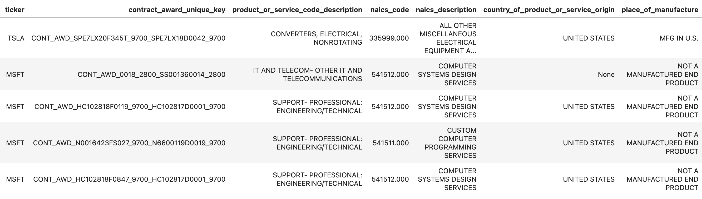
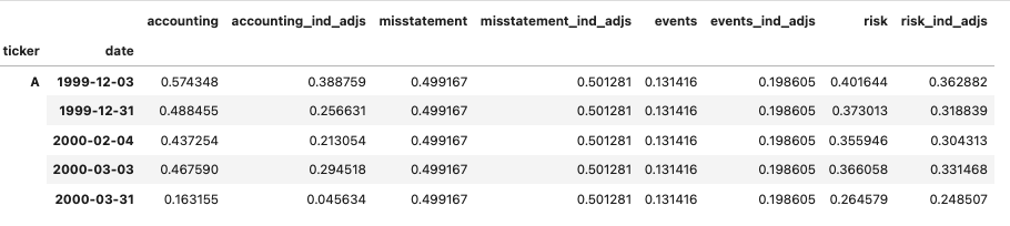
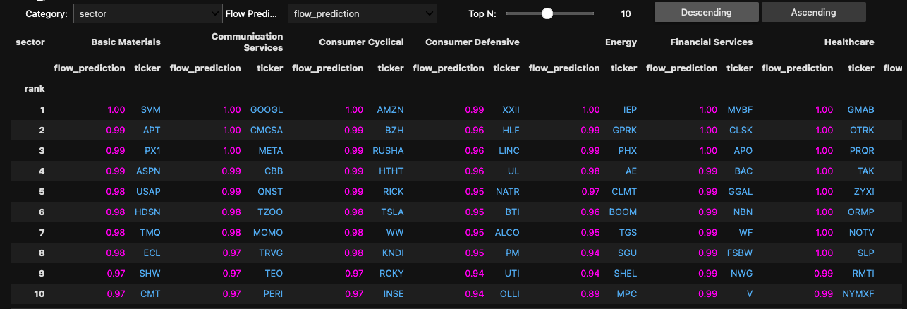
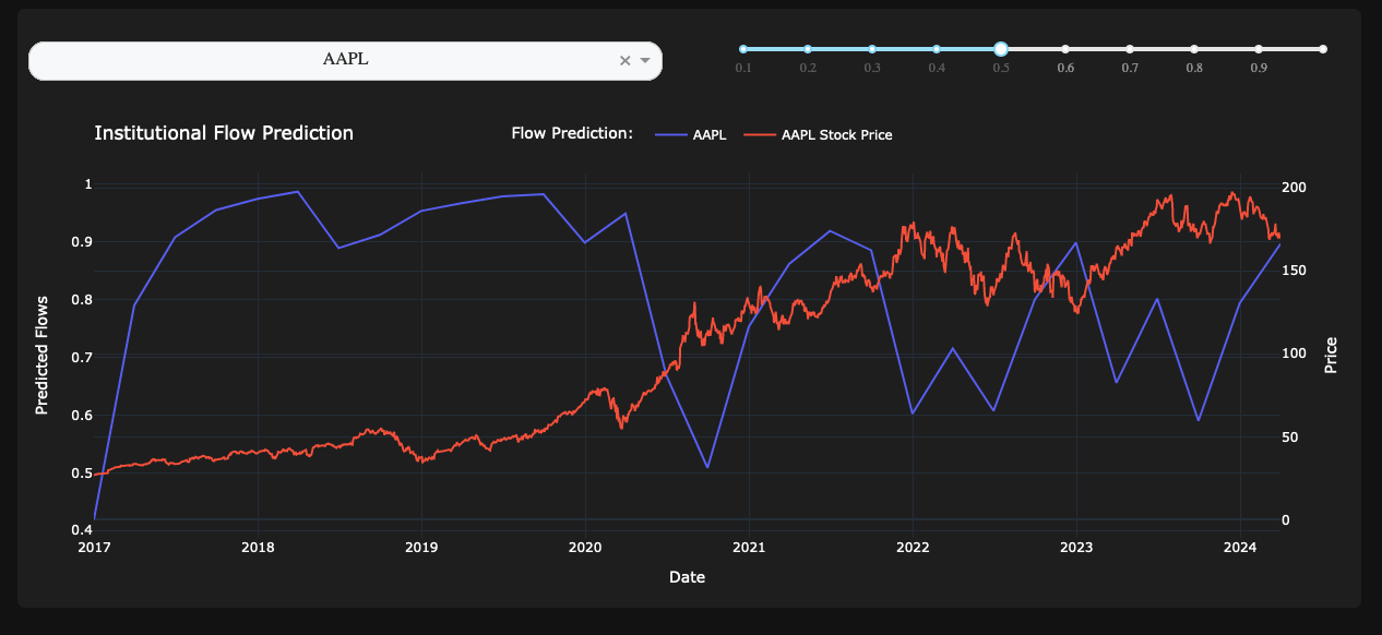
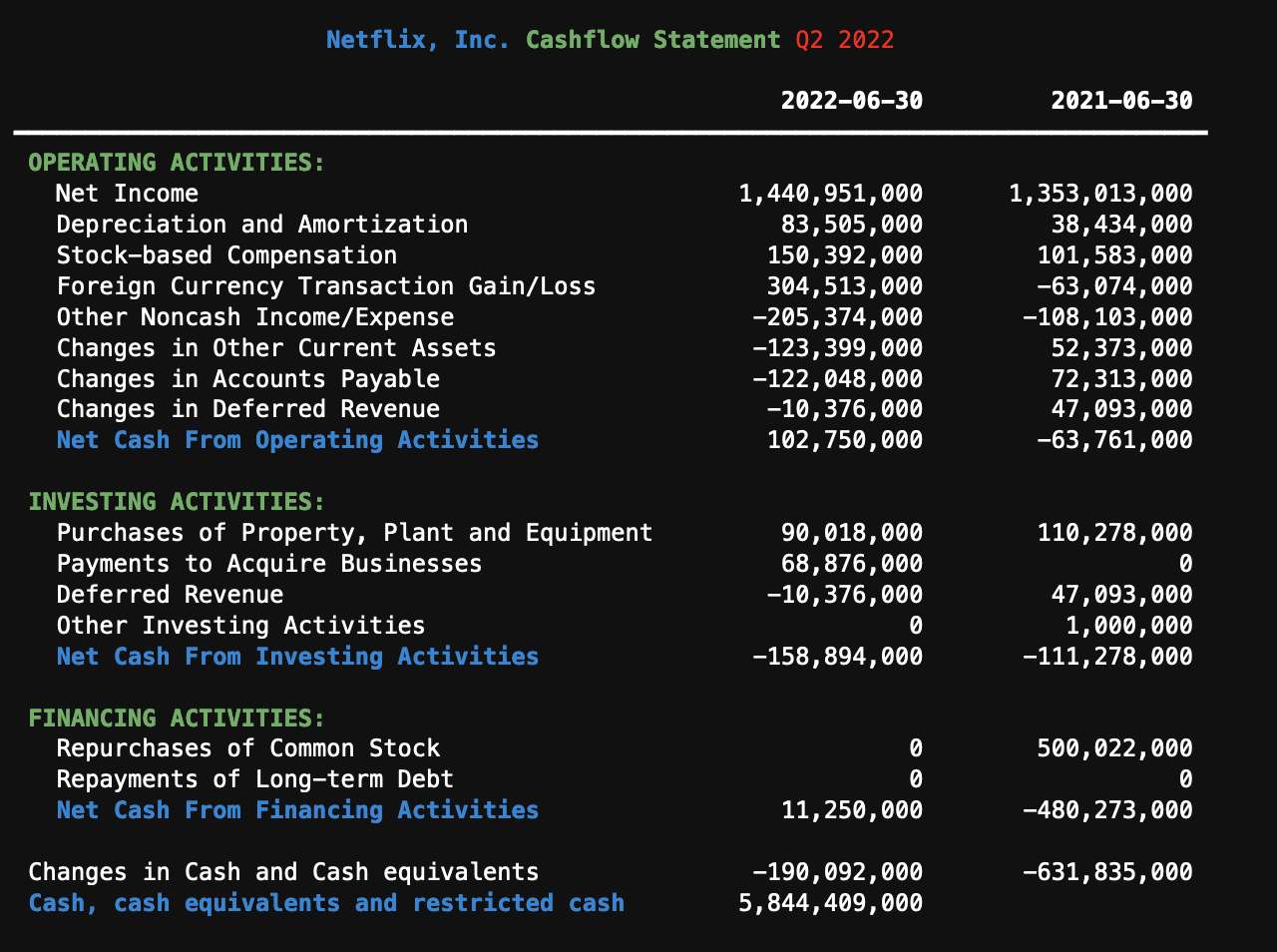
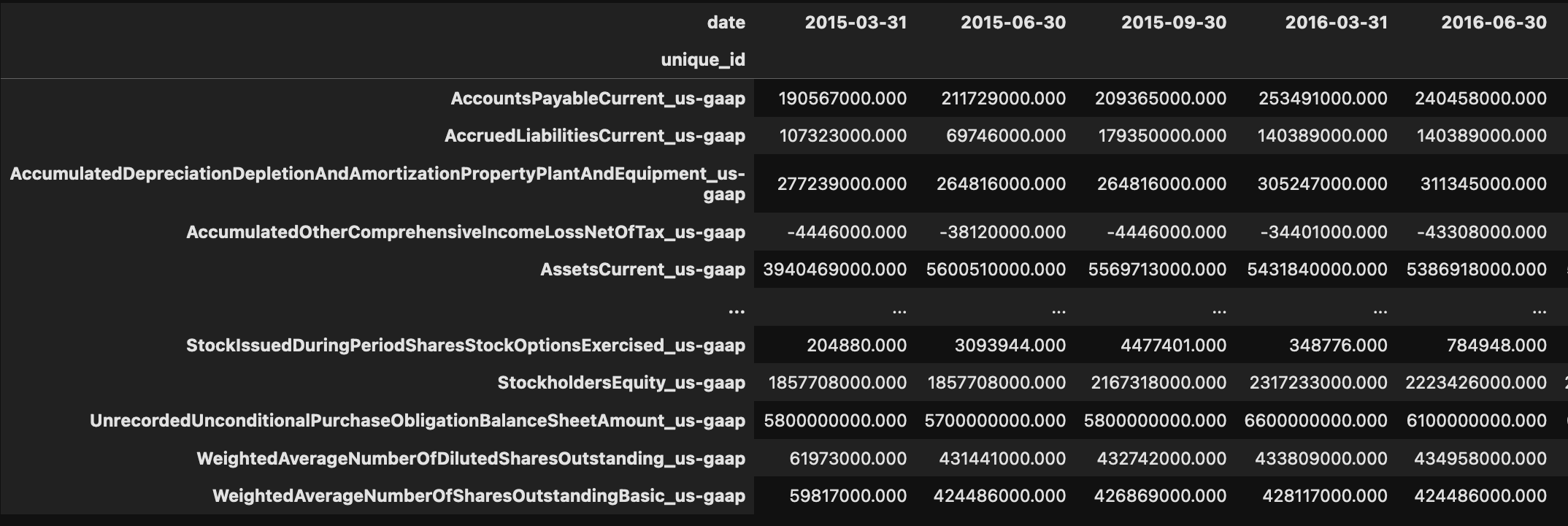
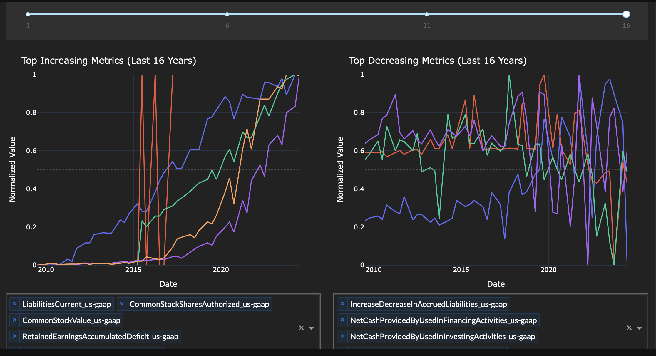
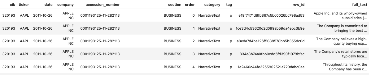
# Data & Screens

**Only works for paying subscribers, purchase your API key** [<mark style="color:purple;">**`here`**</mark>](https://sov.ai/subscribe)**.**

<pre class="language-python"><code class="lang-python">import sovai as sov
<strong>sov.token_auth(token="add_your_subscriber_token_here")
</strong></code></pre>

## Installation

To use Sovai's python module you can install `sovai`.

```
pip install sovai[full]
```

{% hint style="success" %}
**The best way to familiarize yourself with this powerful library is to head straight to the**[ **tutorial section.**](/get-started/tutorials)
{% endhint %}

### Data

If you only want to download data into pandas please use the much lighter package.

```
pip install sovai
```

```python
import sovai as sov
sov.data("query")
```

### Provided Datasets

1. [Equity Datasets](/realtime-datasets/equity-datasets) - Data on publicly traded companies.
2. [Economic Datasets](/realtime-datasets/equity-datasets) - Data for economic forecasting.
3. [Sectorial Datasets](/realtime-datasets/sectorial-datasets) - Sector-specific data for predictive insights.

### Get Help

* The fastest way to get help is to email us at <d.snow@sov.ai> for support.
* We also have a pretty active [Linkedin](https://www.linkedin.com/company/sovai/) page.

## Support us

:tada: For future use, star our [GitHub](https://github.com/sovai-research/sovai-public) repository (click the star button on the top right corner)


# Quick Start

**Only works for paying subscribers, purchase your API key** [<mark style="color:purple;">**`here`**</mark>](https://sov.ai/subscribe)**.**

<pre class="language-python"><code class="lang-python"><strong>import sovai as sov
</strong><strong>sov.token_auth(token="add_your_subscriber_token_here")
</strong></code></pre>

## Installation

To use Sovai's python module you can install `sovai`.

```
pip install sovai[full]
```

{% hint style="success" %}
**The best way to familiarize yourself with this powerful library is to head straight to the**[ **tutorial section.**](/get-started/tutorials)
{% endhint %}

### Data

If you only want to download data into pandas please use the much lighter package.

```
pip install sovai
```

```python
import sovai as sov
sov.data("query")
```

## Commands

Utilize various commands to interact with datasets:, [`data`](#download-datasets) ,[`plots`](#visualizing-data), and [`reports`](#running-reports)`.`

* `sov.data('query')`: Retrieve data based on the specified query.
* `sov.plots('query')`: Generate plots for visual analysis.
* `sov.reports('query')`: Access reports summarizing predictions.

## Authenticate Account: <mark style="color:blue;">`token_auth()`</mark>

There are two ways to authenticate your requests. Get your token [here](https://sov.ai/home).

<pre class="language-python"><code class="lang-python">import sovai as sov

# 1. Method 1: Configuration API connection
<strong>sov.token_auth(token="add_your_token_here")
</strong>
# 2. Method 2: Or read token from .env file e.g API_TOKEN=super_secret_token
sov.read_key('.env')
</code></pre>

## Download Data: : <mark style="color:blue;">`data()`</mark>

Once authenticated, downloading datasets becomes easy.

```python
# Example data retrieval
gs_df = sov.data("bankruptcy/monthly")
```

## Visualize Data: <mark style="color:blue;">`plot()`</mark>

#### Unique Plots

Certain datasets have unique visualizations that you access from their respective pages.

```python
# Calls the 'bankruptcy' dataset and the associated chart_type
sov.plot('bankruptcy', chart_type='compare')
```

#### Universal Plots

Other datasets can use panda's built-in plots.

```python
df_risks = sov.data("risks")
df_risks[["MARKET_RISK","TURING_RISK"]].tail(15400).plot()
```

## Running Reports: <mark style="color:blue;">`report()`</mark>

Run report to explore the dataset.

```python
sov.report("corprisk/accounting",report_type="sector-top")
```

We can also make use of pandas' built-in functions to run queries on top of the data.

```python
df_risks.query("ticker == 'CGRNQ'")
```


# Tutorials

Here are markdown tables with links to the Google Colab, GitHub notebooks, and Jupyter Lab for each tutorial.

## [Datasets](/realtime-datasets/equity-datasets)

<table><thead><tr><th width="244">Tutorial</th><th width="180">Google Colab</th><th>GitHub</th><th>Jupyter Lab</th></tr></thead><tbody><tr><td>Accounting Data</td><td><a href="https://colab.research.google.com/github/sovai-research/sovai-public/blob/main/notebooks/datasets/Accounting%20Data.ipynb">Link</a></td><td><a href="https://github.com/sovai-research/sovai-public/blob/main/notebooks/datasets/Accounting%20Data.ipynb">Link</a></td><td><a href="https://hub.sov.ai/hub/user-redirect/lab/tree/sovai-public/notebooks/datasets/Accounting%20Data.ipynb">Link</a></td></tr><tr><td>Asset Rotation and Allocation</td><td><a href="https://colab.research.google.com/github/sovai-research/sovai-public/blob/main/notebooks/datasets/Asset%20Rotation%20and%20Allocation.ipynb">Link</a></td><td><a href="https://github.com/sovai-research/sovai-public/blob/main/notebooks/datasets/Asset%20Rotation%20and%20Allocation.ipynb">Link</a></td><td><a href="https://hub.sov.ai/hub/user-redirect/lab/tree/sovai-public/notebooks/datasets/Asset%20Rotation%20and%20Allocation.ipynb">Link</a></td></tr><tr><td>Bankruptcy Prediction</td><td><a href="https://colab.research.google.com/github/sovai-research/sovai-public/blob/main/notebooks/datasets/Bankruptcy%20Prediction.ipynb">Link</a></td><td><a href="https://github.com/sovai-research/sovai-public/blob/main/notebooks/datasets/Bankruptcy%20Prediction.ipynb">Link</a></td><td><a href="https://hub.sov.ai/hub/user-redirect/lab/tree/sovai-public/notebooks/datasets/Bankruptcy%20Prediction.ipynb">Link</a></td></tr><tr><td>Breakout Prediction</td><td><a href="https://colab.research.google.com/github/sovai-research/sovai-public/blob/main/notebooks/datasets/Breakout%20Prediction.ipynb">Link</a></td><td><a href="https://github.com/sovai-research/sovai-public/blob/main/notebooks/datasets/Breakout%20Prediction.ipynb">Link</a></td><td><a href="https://hub.sov.ai/hub/user-redirect/lab/tree/sovai-public/notebooks/datasets/Breakout%20Prediction.ipynb">Link</a></td></tr><tr><td>Clinical Trials</td><td><a href="https://colab.research.google.com/github/sovai-research/sovai-public/blob/main/notebooks/datasets/Clinical%20Trials.ipynb">Link</a></td><td><a href="https://github.com/sovai-research/sovai-public/blob/main/notebooks/datasets/Clinical%20Trials.ipynb">Link</a></td><td><a href="https://hub.sov.ai/hub/user-redirect/lab/tree/sovai-public/notebooks/datasets/Clinical%20Trials.ipynb">Link</a></td></tr><tr><td>Congressional Data</td><td><a href="https://colab.research.google.com/github/sovai-research/sovai-public/blob/main/notebooks/datasets/Congressional%20Trading.ipynb">Link</a></td><td><a href="https://github.com/sovai-research/sovai-public/blob/main/notebooks/datasets/Congressional%20Trading.ipynb">Link</a></td><td><a href="https://hub.sov.ai/hub/user-redirect/lab/tree/sovai-public/notebooks/datasets/Congressional%20Trading.ipynb">Link</a></td></tr><tr><td>Consumer Financial Complaints</td><td><a href="https://colab.research.google.com/github/sovai-research/sovai-public/blob/main/notebooks/datasets/Consumer%20Financial%20Complaints.ipynb">Link</a></td><td><a href="https://github.com/sovai-research/sovai-public/blob/main/notebooks/datasets/Consumer%20Financial%20Complaints.ipynb">Link</a></td><td><a href="https://hub.sov.ai/hub/user-redirect/lab/tree/sovai-public/notebooks/datasets/Consumer%20Financial%20Complaints.ipynb">Link</a></td></tr><tr><td>Core Economic Data</td><td><a href="https://colab.research.google.com/github/sovai-research/sovai-public/blob/main/notebooks/datasets/Core%20Economic%20Data.ipynb">Link</a></td><td><a href="https://github.com/sovai-research/sovai-public/blob/main/notebooks/datasets/Core%20Economic%20Data.ipynb">Link</a></td><td><a href="https://hub.sov.ai/hub/user-redirect/lab/tree/sovai-public/notebooks/datasets/Core%20Economic%20Data.ipynb">Link</a></td></tr><tr><td>Corporate Risk Analysis</td><td><a href="https://colab.research.google.com/github/sovai-research/sovai-public/blob/main/notebooks/datasets/Corporate%20Risk%20Analysis.ipynb">Link</a></td><td><a href="https://github.com/sovai-research/sovai-public/blob/main/notebooks/datasets/Corporate%20Risk%20Analysis.ipynb">Link</a></td><td><a href="https://hub.sov.ai/hub/user-redirect/lab/tree/sovai-public/notebooks/datasets/Corporate%20Risk%20Analysis.ipynb">Link</a></td></tr><tr><td>Earnings Surprise</td><td><a href="https://colab.research.google.com/github/sovai-research/sovai-public/blob/main/notebooks/datasets/Earnings%20Surprise.ipynb">Link</a></td><td><a href="https://github.com/sovai-research/sovai-public/blob/main/notebooks/datasets/Earnings%20Surprise.ipynb">Link</a></td><td><a href="https://hub.sov.ai/hub/user-redirect/lab/tree/sovai-public/notebooks/datasets/Earnings%20Surprise.ipynb">Link</a></td></tr><tr><td>Employee Visa</td><td><a href="https://colab.research.google.com/github/sovai-research/sovai-public/blob/main/notebooks/datasets/Employee%20Visa.ipynb">Link</a></td><td><a href="https://github.com/sovai-research/sovai-public/blob/main/notebooks/datasets/Employee%20Visa.ipynb">Link</a></td><td><a href="https://hub.sov.ai/hub/user-redirect/lab/tree/sovai-public/notebooks/datasets/Employee%20Visa.ipynb">Link</a></td></tr><tr><td>Factor Model</td><td><a href="https://colab.research.google.com/github/sovai-research/sovai-public/blob/main/notebooks/datasets/Factor%20Model.ipynb">Link</a></td><td><a href="https://github.com/sovai-research/sovai-public/blob/main/notebooks/datasets/Factor%20Model.ipynb">Link</a></td><td><a href="https://hub.sov.ai/hub/user-redirect/lab/tree/sovai-public/notebooks/datasets/Factor%20Model.ipynb">Link</a></td></tr><tr><td>Financial Ratios</td><td><a href="https://colab.research.google.com/github/sovai-research/sovai-public/blob/main/notebooks/datasets/Financial%20Ratios.ipynb">Link</a></td><td><a href="https://github.com/sovai-research/sovai-public/blob/main/notebooks/datasets/Financial%20Ratios.ipynb">Link</a></td><td><a href="https://hub.sov.ai/hub/user-redirect/lab/tree/sovai-public/notebooks/datasets/Financial%20Ratios.ipynb">Link</a></td></tr><tr><td>Government Web Traffic</td><td><a href="https://colab.research.google.com/github/sovai-research/sovai-public/blob/main/notebooks/datasets/Government%20Internet.ipynb">Link</a></td><td><a href="https://github.com/sovai-research/sovai-public/blob/main/notebooks/datasets/Government%20Internet.ipynb">Link</a></td><td><a href="https://hub.sov.ai/hub/user-redirect/lab/tree/sovai-public/notebooks/datasets/Government%20Internet.ipynb">Link</a></td></tr><tr><td>Government Spending</td><td><a href="https://colab.research.google.com/github/sovai-research/sovai-public/blob/main/notebooks/datasets/Government%20Spending.ipynb">Link</a></td><td><a href="https://github.com/sovai-research/sovai-public/blob/main/notebooks/datasets/Government%20Spending.ipynb">Link</a></td><td><a href="https://hub.sov.ai/hub/user-redirect/lab/tree/sovai-public/notebooks/datasets/Government%20Spending.ipynb">Link</a></td></tr><tr><td>Insider Trading</td><td><a href="https://colab.research.google.com/github/sovai-research/sovai-public/blob/main/notebooks/datasets/Insider%20Trading.ipynb">Link</a></td><td><a href="https://github.com/sovai-research/sovai-public/blob/main/notebooks/datasets/Insider%20Trading.ipynb">Link</a></td><td><a href="https://hub.sov.ai/hub/user-redirect/lab/tree/sovai-public/notebooks/datasets/Insider%20Trading.ipynb">Link</a></td></tr><tr><td>Institutional Holdings</td><td><a href="https://colab.research.google.com/github/sovai-research/sovai-public/blob/main/notebooks/datasets/Insitutional%20Holdings.ipynb">Link</a></td><td><a href="https://github.com/sovai-research/sovai-public/blob/main/notebooks/datasets/Insitutional%20Holdings.ipynb">Link</a></td><td><a href="https://hub.sov.ai/hub/user-redirect/lab/tree/sovai-public/notebooks/datasets/Insitutional%20Holdings.ipynb">Link</a></td></tr><tr><td>Liquidity Data</td><td><a href="https://colab.research.google.com/github/sovai-research/sovai-public/blob/main/notebooks/datasets/Liquidity%20Data.ipynb">Link</a></td><td><a href="https://github.com/sovai-research/sovai-public/blob/main/notebooks/datasets/Liquidity%20Data.ipynb">Link</a></td><td><a href="https://hub.sov.ai/hub/user-redirect/lab/tree/sovai-public/notebooks/datasets/Liquidity%20Data.ipynb">Link</a></td></tr><tr><td>Lobbying Analysis</td><td><a href="https://colab.research.google.com/github/sovai-research/sovai-public/blob/main/notebooks/datasets/Lobbying%20Analysis.ipynb">Link</a></td><td><a href="https://github.com/sovai-research/sovai-public/blob/main/notebooks/datasets/Lobbying%20Analysis.ipynb">Link</a></td><td><a href="https://hub.sov.ai/hub/user-redirect/lab/tree/sovai-public/notebooks/datasets/Lobbying%20Analysis.ipynb">Link</a></td></tr><tr><td>Movies Box Office</td><td><a href="https://colab.research.google.com/github/sovai-research/sovai-public/blob/main/notebooks/datasets/Movies%20Box%20Office.ipynb">Link</a></td><td><a href="https://github.com/sovai-research/sovai-public/blob/main/notebooks/datasets/Movies%20Box%20Office.ipynb">Link</a></td><td><a href="https://hub.sov.ai/hub/user-redirect/lab/tree/sovai-public/notebooks/datasets/Movies%20Box%20Office.ipynb">Link</a></td></tr><tr><td>News</td><td><a href="https://colab.research.google.com/github/sovai-research/sovai-public/blob/main/notebooks/datasets/News.ipynb">Link</a></td><td><a href="https://github.com/sovai-research/sovai-public/blob/main/notebooks/datasets/News.ipynb">Link</a></td><td><a href="https://hub.sov.ai/hub/user-redirect/lab/tree/sovai-public/notebooks/datasets/News.ipynb">Link</a></td></tr><tr><td>Pricing and Market Data</td><td><a href="https://colab.research.google.com/github/sovai-research/sovai-public/blob/main/notebooks/datasets/Pricing%20and%20Market%20Data.ipynb">Link</a></td><td><a href="https://github.com/sovai-research/sovai-public/blob/main/notebooks/datasets/Pricing%20and%20Market%20Data.ipynb">Link</a></td><td><a href="https://hub.sov.ai/hub/user-redirect/lab/tree/sovai-public/notebooks/datasets/Pricing%20and%20Market%20Data.ipynb">Link</a></td></tr><tr><td>Short Data</td><td><a href="https://colab.research.google.com/github/sovai-research/sovai-public/blob/main/notebooks/datasets/Short%20Data.ipynb">Link</a></td><td><a href="https://github.com/sovai-research/sovai-public/blob/main/notebooks/datasets/Short%20Data.ipynb">Link</a></td><td><a href="https://hub.sov.ai/hub/user-redirect/lab/tree/sovai-public/notebooks/datasets/Short%20Data.ipynb">Link</a></td></tr><tr><td>Turing Risk Index</td><td><a href="https://colab.research.google.com/github/sovai-research/sovai-public/blob/main/notebooks/datasets/Turing%20Risk%20Index.ipynb">Link</a></td><td><a href="https://github.com/sovai-research/sovai-public/blob/main/notebooks/datasets/Turing%20Risk%20Index.ipynb">Link</a></td><td><a href="https://hub.sov.ai/hub/user-redirect/lab/tree/sovai-public/notebooks/datasets/Turing%20Risk%20Index.ipynb">Link</a></td></tr><tr><td>Website Traffic</td><td><a href="https://colab.research.google.com/github/sovai-research/sovai-public/blob/main/notebooks/datasets/Website%20Traffic.ipynb">Link</a></td><td><a href="https://github.com/sovai-research/sovai-public/blob/main/notebooks/datasets/Website%20Traffic.ipynb">Link</a></td><td><a href="https://hub.sov.ai/hub/user-redirect/lab/tree/sovai-public/notebooks/datasets/Website%20Traffic.ipynb">Link</a></td></tr><tr><td>Wikipedia</td><td><a href="https://colab.research.google.com/github/sovai-research/sovai-public/blob/main/notebooks/datasets/Wikipedia.ipynb">Link</a></td><td><a href="https://github.com/sovai-research/sovai-public/blob/main/notebooks/datasets/Wikipedia.ipynb">Link</a></td><td><a href="https://hub.sov.ai/hub/user-redirect/lab/tree/sovai-public/notebooks/datasets/Wikipedia.ipynb">Link</a></td></tr></tbody></table>

## Computational

<table><thead><tr><th width="256">Tutorial</th><th width="166">Google Colab</th><th width="167">GitHub</th><th>Jupyter Lab</th></tr></thead><tbody><tr><td>Anomaly Detection</td><td><a href="https://colab.research.google.com/github/sovai-research/sovai-public/blob/main/notebooks/computational/Anomaly%20Detection.ipynb">Link</a></td><td><a href="https://github.com/sovai-research/sovai-public/blob/main/notebooks/computational/Anomaly%20Detection.ipynb">Link</a></td><td><a href="https://hub.sov.ai/hub/user-redirect/lab/tree/sovai-public/notebooks/computational/Anomaly%20Detection.ipynb">Link</a></td></tr><tr><td>Causal Discovery</td><td><a href="https://colab.research.google.com/github/sovai-research/sovai-public/blob/main/notebooks/computational/Causal%20Discovery%20Notebook.ipynb">Link</a></td><td><a href="https://github.com/sovai-research/sovai-public/blob/main/notebooks/computational/Causal%20Discovery%20Notebook.ipynb">Link</a></td><td><a href="https://hub.sov.ai/hub/user-redirect/lab/tree/sovai-public/notebooks/computational/Causal%20Discovery%20Notebook.ipynb">Link</a></td></tr><tr><td>Clustering</td><td><a href="https://colab.research.google.com/github/sovai-research/sovai-public/blob/main/notebooks/computational/Clustering%20Notebook.ipynb">Link</a></td><td><a href="https://github.com/sovai-research/sovai-public/blob/main/notebooks/computational/Clustering%20Notebook.ipynb">Link</a></td><td><a href="https://hub.sov.ai/hub/user-redirect/lab/tree/sovai-public/notebooks/computational/Clustering%20Notebook.ipynb">Link</a></td></tr><tr><td>Decomposition</td><td><a href="https://colab.research.google.com/github/sovai-research/sovai-public/blob/main/notebooks/computational/Decomposition%20Notebook.ipynb">Link</a></td><td><a href="https://github.com/sovai-research/sovai-public/blob/main/notebooks/computational/Decomposition%20Notebook.ipynb">Link</a></td><td><a href="https://hub.sov.ai/hub/user-redirect/lab/tree/sovai-public/notebooks/computational/Decomposition%20Notebook.ipynb">Link</a></td></tr><tr><td>Dimensionality Reduction</td><td><a href="https://colab.research.google.com/github/sovai-research/sovai-public/blob/main/notebooks/computational/Dimensionality%20Reduction.ipynb">Link</a></td><td><a href="https://github.com/sovai-research/sovai-public/blob/main/notebooks/computational/Dimensionality%20Reduction.ipynb">Link</a></td><td><a href="https://hub.sov.ai/hub/user-redirect/lab/tree/sovai-public/notebooks/computational/Dimensionality%20Reduction.ipynb">Link</a></td></tr><tr><td>Feature Extractions</td><td><a href="https://colab.research.google.com/github/sovai-research/sovai-public/blob/main/notebooks/computational/Feature%20Extractions.ipynb">Link</a></td><td><a href="https://github.com/sovai-research/sovai-public/blob/main/notebooks/computational/Feature%20Extractions.ipynb">Link</a></td><td><a href="https://hub.sov.ai/hub/user-redirect/lab/tree/sovai-public/notebooks/computational/Feature%20Extractions.ipynb">Link</a></td></tr><tr><td>Feature Importance</td><td><a href="https://colab.research.google.com/github/sovai-research/sovai-public/blob/main/notebooks/computational/Feature%20Importance.ipynb">Link</a></td><td><a href="https://github.com/sovai-research/sovai-public/blob/main/notebooks/computational/Feature%20Importance.ipynb">Link</a></td><td><a href="https://hub.sov.ai/hub/user-redirect/lab/tree/sovai-public/notebooks/computational/Feature%20Importance.ipynb">Link</a></td></tr><tr><td>Feature Neutralization</td><td><a href="https://colab.research.google.com/github/sovai-research/sovai-public/blob/main/notebooks/computational/Feature%20Neutralization.ipynb">Link</a></td><td><a href="https://github.com/sovai-research/sovai-public/blob/main/notebooks/computational/Feature%20Neutralization.ipynb">Link</a></td><td><a href="https://hub.sov.ai/hub/user-redirect/lab/tree/sovai-public/notebooks/computational/Feature%20Neutralization.ipynb">Link</a></td></tr><tr><td>Feature Selection</td><td><a href="https://colab.research.google.com/github/sovai-research/sovai-public/blob/main/notebooks/computational/Feature%20Selection.ipynb">Link</a></td><td><a href="https://github.com/sovai-research/sovai-public/blob/main/notebooks/computational/Feature%20Selection.ipynb">Link</a></td><td><a href="https://hub.sov.ai/hub/user-redirect/lab/tree/sovai-public/notebooks/computational/Feature%20Selection.ipynb">Link</a></td></tr><tr><td>Nowcasting</td><td><a href="https://colab.research.google.com/github/sovai-research/sovai-public/blob/main/notebooks/computational/Nowcasting%20Notebook.ipynb">Link</a></td><td><a href="https://github.com/sovai-research/sovai-public/blob/main/notebooks/computational/Nowcasting%20Notebook.ipynb">Link</a></td><td><a href="https://hub.sov.ai/hub/user-redirect/lab/tree/sovai-public/notebooks/computational/Nowcasting%20Notebook.ipynb">Link</a></td></tr><tr><td>Pairwise Distance</td><td><a href="https://colab.research.google.com/github/sovai-research/sovai-public/blob/main/notebooks/computational/Pairwise%20Distance.ipynb">Link</a></td><td><a href="https://github.com/sovai-research/sovai-public/blob/main/notebooks/computational/Pairwise%20Distance.ipynb">Link</a></td><td><a href="https://hub.sov.ai/hub/user-redirect/lab/tree/sovai-public/notebooks/computational/Pairwise%20Distance.ipynb">Link</a></td></tr><tr><td>Segmentation</td><td><a href="https://colab.research.google.com/github/sovai-research/sovai-public/blob/main/notebooks/computational/Segmentation%20Notebook.ipynb">Link</a></td><td><a href="https://github.com/sovai-research/sovai-public/blob/main/notebooks/computational/Segmentation%20Notebook.ipynb">Link</a></td><td><a href="https://hub.sov.ai/hub/user-redirect/lab/tree/sovai-public/notebooks/computational/Segmentation%20Notebook.ipynb">Link</a></td></tr></tbody></table>

## Studies

<table><thead><tr><th width="256">Tutorial</th><th width="165">Google Colab</th><th width="166">GitHub</th><th>Jupyter Lab</th></tr></thead><tbody><tr><td>Edgar Tools</td><td><a href="https://colab.research.google.com/github/sovai-research/sovai-public/blob/main/notebooks/studies/Edgar%20Tools.ipynb">Link</a></td><td><a href="https://github.com/sovai-research/sovai-public/blob/main/notebooks/studies/Edgar%20Tools.ipynb">Link</a></td><td><a href="https://hub.sov.ai/hub/user-redirect/lab/tree/sovai-public/notebooks/studies/Edgar%20Tools.ipynb">Link</a></td></tr><tr><td>Screens and Filters</td><td><a href="https://colab.research.google.com/github/sovai-research/sovai-public/blob/main/notebooks/studies/Screens%20and%20Filters.ipynb">Link</a></td><td><a href="https://github.com/sovai-research/sovai-public/blob/main/notebooks/studies/Screens%20and%20Filters.ipynb">Link</a></td><td><a href="https://hub.sov.ai/hub/user-redirect/lab/tree/sovai-public/notebooks/studies/Screens%20and%20Filters.ipynb">Link</a></td></tr><tr><td>Signal Evaluation</td><td><a href="https://colab.research.google.com/github/sovai-research/sovai-public/blob/main/notebooks/studies/Signal%20Evaluation.ipynb">Link</a></td><td><a href="https://github.com/sovai-research/sovai-public/blob/main/notebooks/studies/Signal%20Evaluation.ipynb">Link</a></td><td><a href="https://hub.sov.ai/hub/user-redirect/lab/tree/sovai-public/notebooks/studies/Signal%20Evaluation.ipynb">Link</a></td></tr><tr><td>Weight Optimization</td><td><a href="https://colab.research.google.com/github/sovai-research/sovai-public/blob/main/notebooks/studies/Weight%20Optimization.ipynb">Link</a></td><td><a href="https://github.com/sovai-research/sovai-public/blob/main/notebooks/studies/Weight%20Optimization.ipynb">Link</a></td><td><a href="https://hub.sov.ai/hub/user-redirect/lab/tree/sovai-public/notebooks/studies/Weight%20Optimization.ipynb">Link</a></td></tr></tbody></table>

{% hint style="info" %}
Please get in touch (<d.snow@sov.ai>) if you would like to request new tutorials or receive updates.
{% endhint %}


# Installation

## Install

<pre class="language-python"><code class="lang-python"><strong>import sovai as sov
</strong><strong>sov.token_auth(token="add_your_subscriber_token_here")
</strong></code></pre>

### Full package

<pre><code><strong>pip install sovai[full]
</strong></code></pre>

{% hint style="success" %}
**The best way to familiarize yourself with this powerful library is to head straight to the**[ **tutorial section.**](/get-started/tutorials)
{% endhint %}

### Data package

If you only want to download data into pandas please use the much lighter package.

```
pip install sovai
```

```python
import sovai as sov
sov.data("query")
```

## Environment

Sovai is tested and supported on the following 64-bit systems:

* Python 3.6 – 3.11
* Python 3.9 for Ubuntu only
* Ubuntu 16.04 or later
* Windows 7 or later

In order to avoid potential conflicts with other packages, it is strongly recommended to use a virtual environment, e.g. [python3 virtualenv](https://docs.python.org/3/tutorial/venv.html).

```sh
# Create a virtual environment
python -m venv yourenvname

# Activate the virtual environment
source yourenvname/bin/activate  # For Unix/Linux
yourenvname\Scripts\activate  # For Windows

# Install sovai
pip install sovai

# Create notebook kernel
python -m ipykernel install --user --name yourenvname --display-name "display-name"
```

## Dependencies

Default dependencies that are installed with `pip install sovai` are [listed here](https://github.com/sovai-research/SovAI/blob/master/pyproject.toml).

#### Select the tab

{% tabs %}
{% tab title="requirements" %}
numpy>=1.20

scipy>=1.0

pandas>=1.0

python-dateutil>=2.8

python-dotenv>=0.10

requests>=2.20

joblib>=1.0

pyarrow>=5.0

matplotlib>=3.0

plotly>=5.0

scikit-learn>=1.0

numba>=0.50

boto3>=1.20

dash>=2.0

great-tables>=0.9

polars>=0.20.30

ruptures>=1.0

shap>=0.40

skfolio>=0.3

statsforecast>=1.0

tensorly>=0.6

openai>=1.0

mfles>=0.2

pexpect>=4.9.0

lightgbm>=4.5.0

ipywidgets>=8.1.3

polars-talib==0.1.3

dash-bootstrap-components>=1.6.0
{% endtab %}

{% tab title="requirements-dev" %}
poetry>=1.0

pytest>=6.0

flake8>=3.9

black>=21.0

isort>=5.0

mypy>=0.900
{% endtab %}
{% endtabs %}

## Docker

Docker uses containers to create virtual environments that isolate a Sovai installation from the rest of the system. Sovai docker comes pre-installed with a Notebook environment that can share resources with its host machine (access directories, use the GPU, connect to the Internet, etc.). The Sovai Docker images are tested for each release.

```bash
docker run -p 8888:8888 sovai/slim
```

For docker image with full version:

```bash
docker run -p 8888:8888 sovai/full
```


# Release Notes

This page shows release notes >= 0.0

### **Sovai 0.2.6**

**Release Date: April 10, 2024 (BUG FIXES, NEW FUNCTIONALITY)**

* Updated `README.dev.md` with fixes for the auto release action and enhancements to the documentation to improve developer onboarding and usage clarity.
* **License and Setup**: Updated `LICENSE`, `Makefile`, and `requirements.txt` as part of a global refactor, transitioning dependency management to Poetry and reinforcing the testing framework.


# About

SovAI was founded in 2023 to make machine learning solutions accessible to investment managers.

<figure><img src="https://1304136543-files.gitbook.io/~/files/v0/b/gitbook-x-prod.appspot.com/o/spaces%2FCbqQ4ogM0YiEs5Z9Djdn%2Fuploads%2Fgit-blob-0ca6f363d7c552adbb9b8d8104e35bbe620879bf%2Fabout_1.png?alt=media" alt=""><figcaption></figcaption></figure>

The company is privately funded, ensuring the independence and objectivity of its research outputs.

<figure><img src="https://1304136543-files.gitbook.io/~/files/v0/b/gitbook-x-prod.appspot.com/o/spaces%2FCbqQ4ogM0YiEs5Z9Djdn%2Fuploads%2Fgit-blob-a370afe3572ee5c6574e4752fdc092d4498349db%2Fabout_2.png?alt=media" alt=""><figcaption></figcaption></figure>

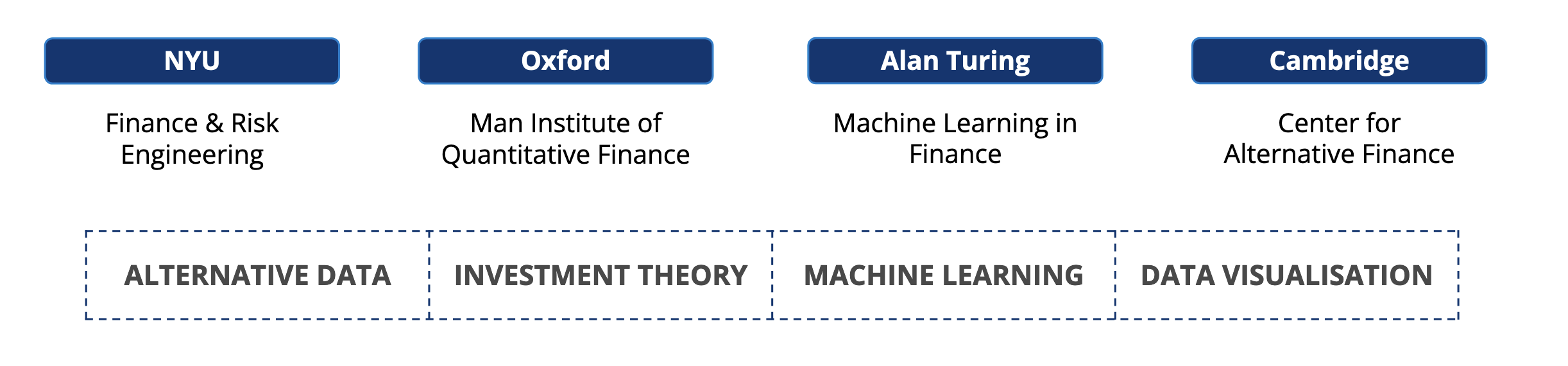
The software is built by alumni from the **Alan Turing Institute**, the Oxford-Man Institute of Quantitative Finance at **Oxford University**, and financial engineering and computer science graduates at **New York University**.

<figure><img src="https://1304136543-files.gitbook.io/~/files/v0/b/gitbook-x-prod.appspot.com/o/spaces%2FCbqQ4ogM0YiEs5Z9Djdn%2Fuploads%2Fgit-blob-6058e5dadc0bb73efba0e3cec06f1e9264754851%2Fabout_3.png?alt=media" alt=""><figcaption></figcaption></figure>

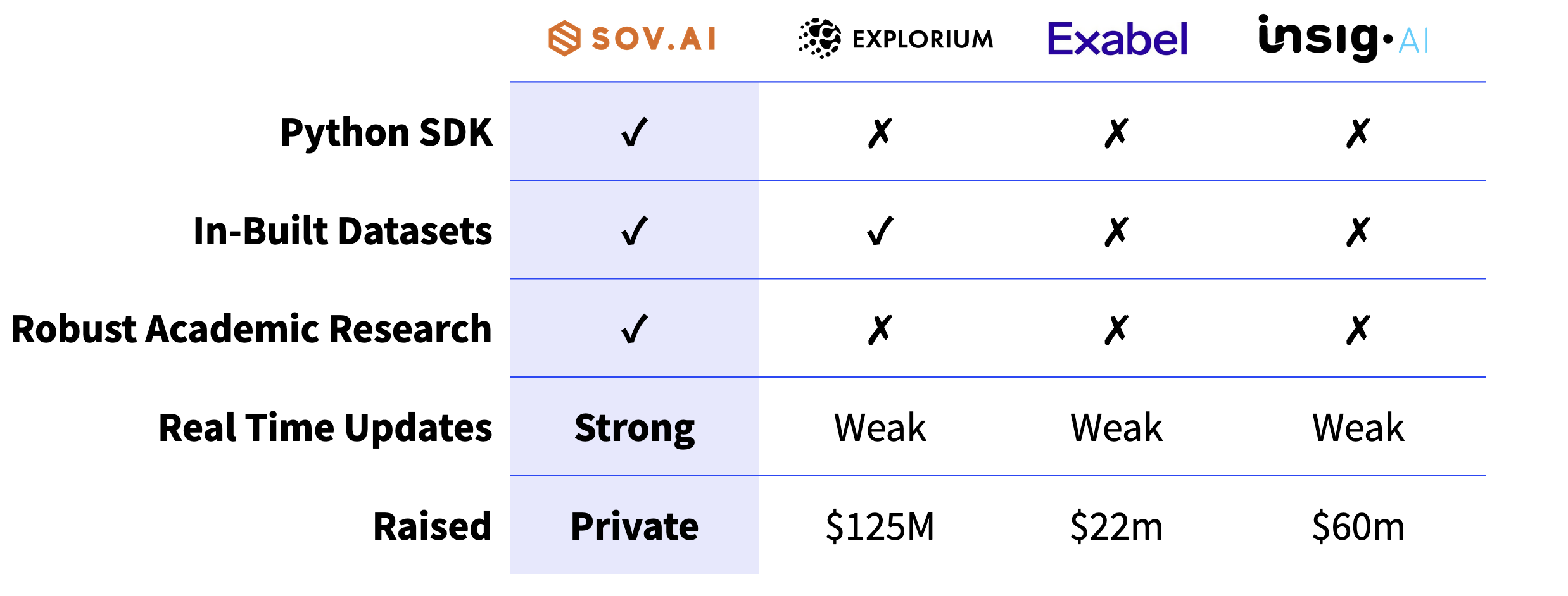
SovAI is and will remain the most robust and most affordable subscription product on the market.

<figure><img src="https://1304136543-files.gitbook.io/~/files/v0/b/gitbook-x-prod.appspot.com/o/spaces%2FCbqQ4ogM0YiEs5Z9Djdn%2Fuploads%2Fgit-blob-f26b64f9c81e3eeb6f9ae2ef335348901cbd9afc%2Fabout_4.png?alt=media" alt=""><figcaption></figcaption></figure>

Finally, we have benefited from the input of the following **four academic advisors** who have been supporting us since the birth of SovAI.

<figure><img src="https://1304136543-files.gitbook.io/~/files/v0/b/gitbook-x-prod.appspot.com/o/spaces%2FCbqQ4ogM0YiEs5Z9Djdn%2Fuploads%2Fgit-blob-e07648e476c5c8fb0cd8a544b79646e2efd64f1b%2Fabout_5.png?alt=media" alt=""><figcaption></figcaption></figure>


# Equity Datasets


# Accounting Data

Standardized financial accounting data across multiple US publicly traded firms.

{% hint style="warning" %}
This dataset is derived from public filings, so we cannot guarantee its quality. Replace with your commercial standardized accounting solution.
{% endhint %}

{% hint style="info" %}
Daily index data is updated before market opens in the US ET time.
{% endhint %}

{% hint style="success" %}
Dataset contains 5250+ tickers, available from 1994-03-11 onwards.
{% endhint %}

`Tutorials` are the best documentation — [<mark style="color:blue;">`Accounting Data Tutorial`</mark>](https://colab.research.google.com/github/sovai-research/sovai-public/blob/main/notebooks/datasets/Accounting%20Data.ipynb)

<table data-column-title-hidden data-view="cards"><thead><tr><th>Category</th><th>Details</th></tr></thead><tbody><tr><td><strong>Input Datasets</strong></td><td>SEC Filings, EDGAR API, Raw XBRL</td></tr><tr><td><strong>Models Used</strong></td><td>Imputation Models, Validation Against Commercial Dataset</td></tr><tr><td><strong>Model Outputs</strong></td><td>Monthly Accounting Values</td></tr></tbody></table>

## Description

This dataset provides standardized financial accounting data for US publicly traded companies, compiled from SEC filings and validated against commercial datasets.

It offers a comprehensive view of companies' financial positions and performance, including balance sheet, income statement, and cash flow data, making it valuable for investors conducting financial analysis and quantitative modeling.

## Data Access

### Retrieving Data

#### Ticker Data

```python
import sovai as sov
df_accounting = sov.data("accounting/weekly", tickers=["MSFT", "TSLA", "META"])
```

<figure><img src="https://1304136543-files.gitbook.io/~/files/v0/b/gitbook-x-prod.appspot.com/o/spaces%2FCbqQ4ogM0YiEs5Z9Djdn%2Fuploads%2Fgit-blob-711b401eb16875ffc2b9f4f6e0452070b848b66b%2Faccounting_data_1.png?alt=media" alt=""><figcaption></figcaption></figure>

#### Latest Data

```python
import sovai as sov
df_accounting = sov.data("accounting/weekly")
```

#### All Data

```python
import sovai as sov
df_accounting = sov.data("accounting/weekly", full_history=True)
```

## Reports

### Balance Sheet Report

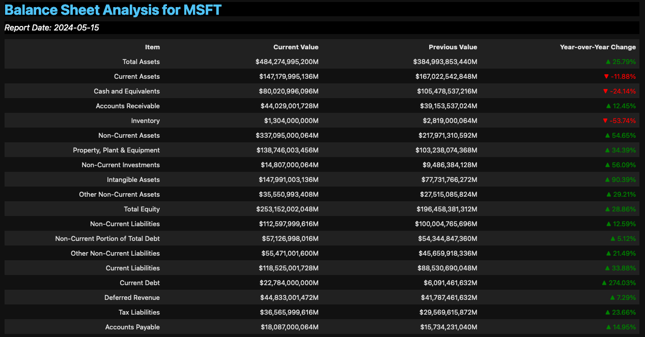
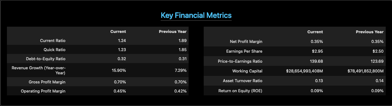
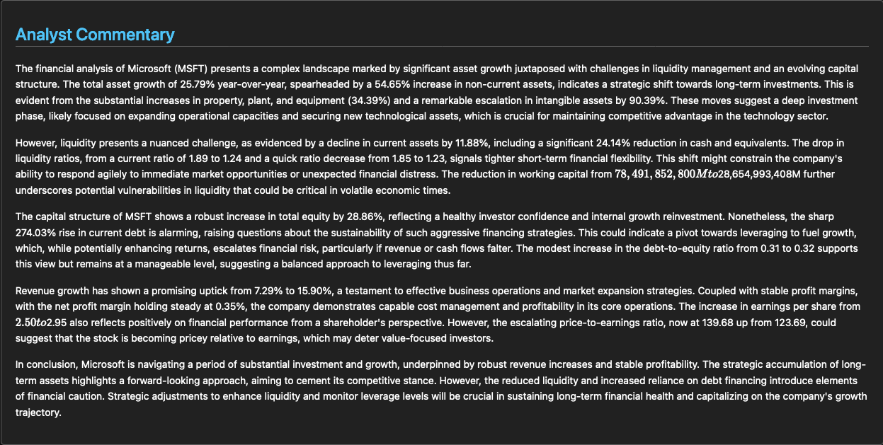
```python
import sovai as sov
sov.report("accounting", report_type="balance_sheet", ticker="MSFT")
```

<figure><img src="https://1304136543-files.gitbook.io/~/files/v0/b/gitbook-x-prod.appspot.com/o/spaces%2FCbqQ4ogM0YiEs5Z9Djdn%2Fuploads%2Fgit-blob-dea7fcae49f782d752710030a734448253e76599%2Faccounting_data_2.png?alt=media" alt=""><figcaption></figcaption></figure>

<figure><img src="https://1304136543-files.gitbook.io/~/files/v0/b/gitbook-x-prod.appspot.com/o/spaces%2FCbqQ4ogM0YiEs5Z9Djdn%2Fuploads%2Fgit-blob-4a71a8f17bd03130ecf6570c4a63d4544372fb8f%2Faccounting_data_3.png?alt=media" alt=""><figcaption></figcaption></figure>

<figure><img src="https://1304136543-files.gitbook.io/~/files/v0/b/gitbook-x-prod.appspot.com/o/spaces%2FCbqQ4ogM0YiEs5Z9Djdn%2Fuploads%2Fgit-blob-800e7a6aa106942613c024dc5f9eab6e2fbcd479%2Faccounting_data_4.png?alt=media" alt=""><figcaption></figcaption></figure>

## Plots

### Tree Plot

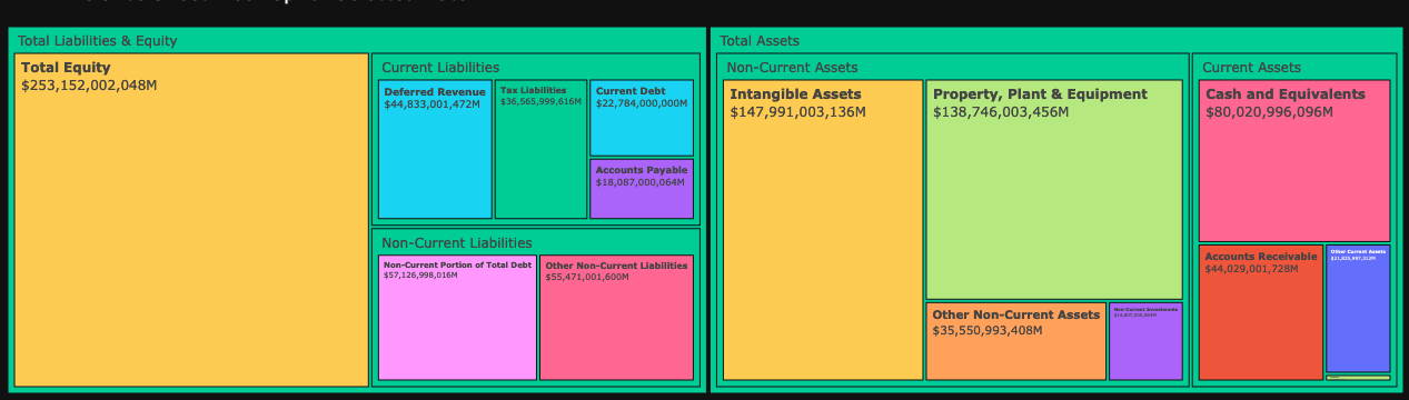
```python
import sovai as sov
sov.plot("accounting", chart_type="balance", ticker="MSFT")
```

<figure><img src="https://1304136543-files.gitbook.io/~/files/v0/b/gitbook-x-prod.appspot.com/o/spaces%2FCbqQ4ogM0YiEs5Z9Djdn%2Fuploads%2Fgit-blob-3b6fbd1d96c793d886d81b9c9bee69a58680b307%2Faccounting_data_5.png?alt=media" alt=""><figcaption></figcaption></figure>

## Data Dictionary

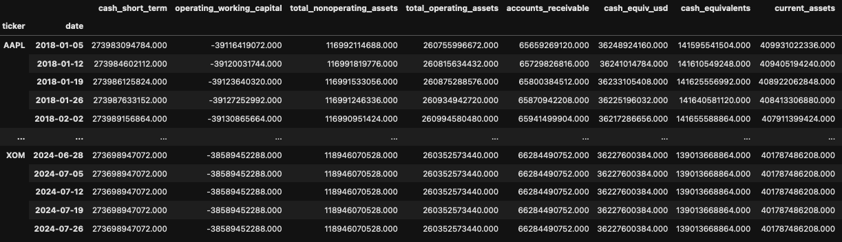
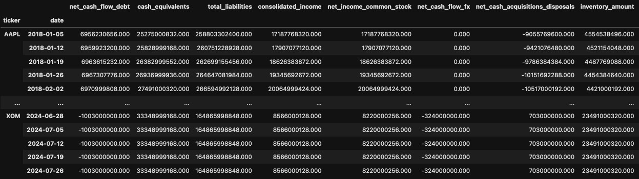
<table><thead><tr><th width="204">name</th><th width="318">description</th><th width="130">domain</th><th width="140">characteristic</th></tr></thead><tbody><tr><td>working_capital</td><td>Working capital is the net amount of [current_assets] minus [current_liabilities], giving an indication of the short-term financial health of a company.</td><td>Metrics</td><td>Assets</td></tr><tr><td>ticker</td><td>A ticker symbol, often referred to as a stock symbol, is a unique [entity] that identifies a publicly traded security in financial markets</td><td>Entity</td><td>Entity</td></tr><tr><td>tax_liabilities</td><td>On the [balance sheet], this line item represents the total amount of tax obligations due, included within [total_liabilities], that the company is responsible for paying</td><td>Balance Sheet</td><td>Liabilities</td></tr><tr><td>tax_expenses</td><td>This represents the sum of current and deferred income tax expenses related to ongoing operations, as reported on the [income statement]. It reflects the company's tax liabilities for the period.</td><td>Income Statement</td><td>Expense</td></tr><tr><td>tax_assets</td><td>Tax assets, listed on the [balance sheet], include all tax-related receivables and potential tax benefits that are recognized as part of [total_assets].</td><td>Balance Sheet</td><td>Assets</td></tr><tr><td>tangible_assets</td><td>The value of a company's physical assets, or [tangible_assets], is calculated by subtracting [intangible_assets] from [total_assets], as indicated in [metrics].</td><td>Metrics</td><td>Assets</td></tr><tr><td>selling_general_admin_expenses</td><td>This [income statement] entry sums up all costs associated with selling the company's products and managing its operations, excluding production costs. It includes both direct selling expenses and broader administrative costs.</td><td>Income Statement</td><td>Expense</td></tr><tr><td>stock_based_compensation</td><td>This item on the [cash flow statement] reflects compensation given to employees in the form of equity or options, which is considered noncash and therefore added back to net cash from operating activities.</td><td>Cash Flow Statement</td><td>Cash Flow</td></tr><tr><td>research_development_expenses</td><td>This [income statement] line item tallies up all expenses associated with the development of new products or services, reflecting a company's investment in innovation.</td><td>Income Statement</td><td>Expense</td></tr><tr><td>revenue_usd</td><td>This [income statement] figure represents [total_revenue] converted into USD, using the [forex_usd] exchange rate, to standardize international revenue figures.</td><td>Income Statement</td><td>Income</td></tr><tr><td>total_revenue</td><td>The total amount recognized from providing goods and services, as seen on the [income statement], it's a fundamental gauge of the company's financial performance.</td><td>Income Statement</td><td>Income</td></tr><tr><td>retained_earnings</td><td>[balance sheet] Represents the cumulative earnings or deficit that an entity has retained over time as part of [total_equity]. This may be reported annually for some entities.</td><td>Balance Sheet</td><td>Equity</td></tr><tr><td>accounts_receivable</td><td>[balance sheet] Includes all trade and non-trade receivables as part of [total_assets], signifying amounts owed to the entity that are expected to be collected.</td><td>Balance Sheet</td><td>Assets</td></tr><tr><td>preferred_dividends</td><td>[income statement] Reflects dividends paid to preferred stockholders, deducted from [net_income] to determine the earnings available to common stockholders.</td><td>Income Statement</td><td>Expense</td></tr><tr><td>property_plant_equipment_net</td><td>[balance sheet] The net value of a company's investment in physical assets used in operations, net of depreciation and including Operating Right of Use Assets.</td><td>Balance Sheet</td><td>Assets</td></tr><tr><td>accounts_payable</td><td>[balance sheet] Represents amounts the company owes to suppliers and creditors, forming part of [total_liabilities].</td><td>Balance Sheet</td><td>Liabilities</td></tr><tr><td>operating_income</td><td>[income statement] Shows a company's earnings from core operations, derived as [gross_profit] minus [operating_expenses], excluding [interest_expense] and [tax_expenses].</td><td>Income Statement</td><td>Income</td></tr><tr><td>operating_expenses</td><td>[income statement] Encompasses all costs related to the day-to-day functioning of the business, excluding costs directly tied to production ([cost_of_revenue]).</td><td>Income Statement</td><td>Expense</td></tr><tr><td>net_income_non_controlling_int</td><td>[income statement] Reflects the share of earnings allocated to minority shareholders, deducted from [consolidated_income] to arrive at [net_income].</td><td>Income Statement</td><td>Income</td></tr><tr><td>net_income_discontinued_ops</td><td>[income statement] Represents the financial impact of ceasing operations or disposing of a part of the business, shown separately from ongoing operations.</td><td>Income Statement</td><td>Income</td></tr><tr><td>net_income_common_stock_usd</td><td>[income statement] The portion of [net_income_common_stock] presented in USD, converted using [forex_usd].</td><td>Income Statement</td><td>Income</td></tr><tr><td>net_income_common_stock</td><td>[income statement] The total earnings attributable to common shareholders, which may differ from [net_income] due to [preferred_dividends].</td><td>Income Statement</td><td>Income</td></tr><tr><td>net_income</td><td>[income statement] The total earnings or losses for the period attributable to the parent company, after accounting for non-controlling interests and before preferred dividends.</td><td>Income Statement</td><td>Income</td></tr><tr><td>net_cash_flow_fx</td><td>[cash flow statement] Reflects the impact of foreign exchange rate movements on the company's cash and cash equivalents held in different currencies.</td><td>Cash Flow Statement</td><td>Cash Flow</td></tr><tr><td>net_cash_flow_operating</td><td>[cash flow statement] Represents the cash a company generates from its ongoing, regular business activities.</td><td>Cash Flow Statement</td><td>Cash Flow</td></tr><tr><td>net_cash_acquisitions_disposals</td><td>[cash flow statement] Details the cash transactions involved in the company's investment acquisitions and disposals.</td><td>Cash Flow Statement</td><td>Cash Flow</td></tr><tr><td>net_cash_flow_investing</td><td>[cash flow statement] Reflects the cash transactions related to a company's investment activities within [net_cash_flow], including capital expenditures, acquisitions, and disposals.</td><td>Cash Flow Statement</td><td>Cash Flow</td></tr><tr><td>net_cash_flow_financing</td><td>[cash flow statement] Indicates the cash movements from financing activities within [net_cash_flow], including equity transactions, debt servicing, and dividends.</td><td>Cash Flow Statement</td><td>Cash Flow</td></tr><tr><td>net_cash_flow_dividends</td><td>[cash flow statement] Part of [net_cash_flow_financing], this represents the cash distributed to shareholders as dividends.</td><td>Cash Flow Statement</td><td>Cash Flow</td></tr><tr><td>net_cash_flow_debt</td><td>[cash flow statement] Represents the net cash from the issuance and repayment of debt within [net_cash_flow_financing].</td><td>Cash Flow Statement</td><td>Cash Flow</td></tr><tr><td>net_cash_flow_common</td><td>[cash flow statement] Details the cash changes from the sale or purchase of equity within [net_cash_flow_financing].</td><td>Cash Flow Statement</td><td>Cash Flow</td></tr><tr><td>net_cash_flow_business</td><td>[cash flow statement] Describes the net cash impact of buying or selling business units within [net_cash_flow_investing].</td><td>Cash Flow Statement</td><td>Cash Flow</td></tr><tr><td>net_cash_flow</td><td>[cash flow statement] Summarizes the total change in cash and equivalents, accounting for operational, investment, and financial cash flows, as well as foreign exchange effects.</td><td>Cash Flow Statement</td><td>Cash Flow</td></tr><tr><td>non_current_liabilities</td><td>[balance sheet] Represents long-term obligations of the company, which are not due within the next 12 months.</td><td>Balance Sheet</td><td>Liabilities</td></tr><tr><td>current_liabilities</td><td>[balance sheet] Represents obligations of the company due within the next 12 months.</td><td>Balance Sheet</td><td>Liabilities</td></tr><tr><td>total_liabilities</td><td>[balance sheet] The aggregate of all debts and financial obligations due by the company at any point in time.</td><td>Balance Sheet</td><td>Liabilities</td></tr><tr><td>non_current_investments</td><td>[balance sheet] Long-term investments not expected to be liquidated within the next year.</td><td>Balance Sheet</td><td>Assets</td></tr><tr><td>current_investments</td><td>[balance sheet] Short-term investments expected to be liquidated or used within one year.</td><td>Balance Sheet</td><td>Assets</td></tr><tr><td>total_investments</td><td>[balance sheet] Sum of all investments, both marketable securities and loans, reflecting a company's investment holdings.</td><td>Balance Sheet</td><td>Assets</td></tr><tr><td>inventory_amount</td><td>[balance sheet] Value of the company's stock of goods and materials held to be sold or used in production.</td><td>Balance Sheet</td><td>Assets</td></tr><tr><td>invested_capital</td><td>[metrics] Total money invested in a company for generating returns, not considering current obligations and liquid assets.</td><td>Metrics</td><td>Equity</td></tr><tr><td>interest_expense</td><td>[income statement] The total cost incurred by the company for the use of borrowed funds.</td><td>Income Statement</td><td>Expense</td></tr><tr><td>intangible_assets</td><td>[balance sheet] The net worth of non-physical assets like patents and copyrights held by the company.</td><td>Balance Sheet</td><td>Assets</td></tr><tr><td>gross_profit</td><td>[income statement] The profit a company makes after subtracting the costs associated with making and selling its products.</td><td>Income Statement</td><td>Income</td></tr><tr><td>free_cash_flow</td><td>[metrics] An important performance indicator that shows how much cash is generated from operations after subtracting capital expenditures.</td><td>Metrics</td><td>Cash Flow</td></tr><tr><td>enterprise_value</td><td>[metrics] The total valuation of a company, including its equity, debt, and cash holdings.</td><td>Metrics</td><td>Valuation</td></tr><tr><td>equity_usd</td><td>[balance sheet] The company's total equity, converted into USD using the appropriate foreign exchange rate.</td><td>Balance Sheet</td><td>Equity</td></tr><tr><td>total_equity</td><td>[balance sheet] The net value attributable to the parent company, including equity and all receivables from related parties.</td><td>Balance Sheet</td><td>Equity</td></tr><tr><td>earnings_before_tax</td><td>[metrics] The company's earnings calculated before any tax expenses are deducted.</td><td>Metrics</td><td>Profitability</td></tr><tr><td>ebit_usd</td><td>[income statement] The company's earnings before interest and taxes, reported in USD and adjusted for exchange rates.</td><td>Income Statement</td><td>Income</td></tr><tr><td>ebitda</td><td>[metrics] A common profitability measure excluding the non-cash expenses of depreciation and amortization from [ebit].</td><td>Metrics</td><td>Profitability</td></tr><tr><td>ebit</td><td>[income statement] The profit a company makes after all expenses except for interest and taxes have been subtracted from [net_income].</td><td>Income Statement</td><td>Income</td></tr><tr><td>bank_deposits</td><td>[balance sheet] The total of all customer deposits and other types of bank-held liabilities.</td><td>Balance Sheet</td><td>Liabilities</td></tr><tr><td>depreciation_amortization</td><td>[cash flow statement] The total non-cash expenses for asset depreciation, amortization, and accretion recognized during the period.</td><td>Cash Flow Statement</td><td>Cash Flow</td></tr><tr><td>deferred_revenue</td><td>[balance sheet] Income that has been received but not yet earned, and thus not recognized as revenue.</td><td>Balance Sheet</td><td>Liabilities</td></tr><tr><td>debt_usd</td><td>[balance sheet] Represents the total borrowings of a company, converted to USD using the current exchange rate.</td><td>Balance Sheet</td><td>Liabilities</td></tr><tr><td>non_current_debt</td><td>[balance sheet] The portion of [total_debt] that is not due within the next twelve months.</td><td>Balance Sheet</td><td>Liabilities</td></tr><tr><td>current_debt</td><td>[balance sheet] The portion of [total_debt] that is due within the next twelve months.</td><td>Balance Sheet</td><td>Liabilities</td></tr><tr><td>total_debt</td><td>[balance sheet] The aggregate amount of current and long-term borrowing obligations.</td><td>Balance Sheet</td><td>Liabilities</td></tr><tr><td>cost_of_revenue</td><td>[income statement] The total cost incurred to produce the goods or services sold during a specific period.</td><td>Income Statement</td><td>Expense</td></tr><tr><td>consolidated_income</td><td>[income statement] The total earnings for the consolidated entity after taxes but before deducting earnings attributable to non-controlling interests.</td><td>Income Statement</td><td>Income</td></tr><tr><td>cash_equiv_usd</td><td>[balance sheet] The amount of [cash_equivalents] held by a company, expressed in USD and converted using the [forex_usd] rate.</td><td>Balance Sheet</td><td>Assets</td></tr><tr><td>cash_equivalents</td><td>[balance sheet] Cash on hand and in banks, as well as cash equivalents, which are liquid and short-term in nature.</td><td>Balance Sheet</td><td>Assets</td></tr><tr><td>capital_expenditures</td><td>[cash flow statement] Outlays of cash intended to produce long-term benefits, such as purchasing or upgrading physical assets like property, plant, or equipment.</td><td>Cash Flow Statement</td><td>Cash Flow</td></tr><tr><td>non_current_assets</td><td>[balance sheet] The total value of assets that are not expected to be converted to cash within one year.</td><td>Balance Sheet</td><td>Assets</td></tr><tr><td>current_assets</td><td>[balance sheet] Assets that are expected to be converted to cash, sold, or consumed within a year.</td><td>Balance Sheet</td><td>Assets</td></tr><tr><td>total_assets</td><td>[balance sheet] The total value of all recognized assets owned by a company at the end of a reporting period.</td><td>Balance Sheet</td><td>Assets</td></tr><tr><td>accum_other_comp_income</td><td>[balance sheet] The total accumulated amount of income or loss not recognized in net income, including items like foreign currency translation adjustments and unrealized gains/losses on securities.</td><td>Balance Sheet</td><td>Equity</td></tr><tr><td>dividends_total</td><td>Total dividends paid, calculated as dividends per share times shares outstanding.</td><td>Income Statement</td><td>Expense</td></tr><tr><td>cash_short_term</td><td>Sum of cash and short-term investments.</td><td>Balance Sheet</td><td>Asset</td></tr><tr><td>total_operating_net_income</td><td>Combined income from ongoing operations and discontinued operations.</td><td>Income Statement</td><td>Income</td></tr><tr><td>net_income_excluding_discontinued</td><td>Net income with the income from discontinued operations removed.</td><td>Income Statement</td><td>Income</td></tr><tr><td>comprehensive_net_income</td><td>Aggregate net income including all operations and adjustments.</td><td>Income Statement</td><td>Income</td></tr><tr><td>adjusted_parent_equity</td><td>Parent equity adjusted for tax assets and preferred dividends.</td><td>Balance Sheet</td><td>Equity</td></tr><tr><td>book_equity_value</td><td>Final book value of equity after adjustments for invested capital, debt, and investments.</td><td>Balance Sheet</td><td>Equity</td></tr><tr><td>operating_working_capital</td><td>Capital used in the business's ongoing operations.</td><td>Balance Sheet</td><td>Asset</td></tr><tr><td>total_nonoperating_assets</td><td>Assets not directly related to the company's core operations.</td><td>Balance Sheet</td><td>Asset</td></tr><tr><td>operating_accruals</td><td>Accruals related to operating activities, adjusted for net income and cash flow.</td><td>Cash Flow Statement</td><td>Cash Flow</td></tr><tr><td>operating_cash_flow</td><td>Cash flow from operating activities, adjusted for net income and accruals.</td><td>Cash Flow Statement</td><td>Cash Flow</td></tr><tr><td>total_operating_assets</td><td>Total assets attributed to the company's primary business activities.</td><td>Balance Sheet</td><td>Asset</td></tr><tr><td>cash_operating_profit</td><td>Operating profit adjusted for non-cash EBITDA and accruals.</td><td>Income Statement</td><td>Income</td></tr><tr><td>total_accruals</td><td>Total accrual-based adjustments to net income.</td><td>Cash Flow Statement</td><td>Cash Flow</td></tr></tbody></table>

***


# Bankruptcy Predictions

Chapter 7 and Chapter 11 bankruptcy predictions made easy for over 5,000 US publicly traded stocks.

{% hint style="info" %}
Monthly corporate bankruptcy predictions arrive the **2nd of every month***.*
{% endhint %}

{% hint style="success" %}
Dataset contains 4762+ tickers, available from 1998-03-31 onwards.
{% endhint %}

`Tutorials` are the best documentation — [<mark style="color:blue;">`Corporate Bankruptcy Tutorial`</mark>](https://colab.research.google.com/github/sovai-research/sovai-public/blob/main/notebooks/datasets/Bankruptcy%20Prediction.ipynb)

<table data-view="cards" data-full-width="false"><thead><tr><th></th><th></th></tr></thead><tbody><tr><td><strong>Input Datasets</strong></td><td>SEC Bankruptcies, Delistings, Market Data, Financial Statements</td></tr><tr><td><strong>Models Used</strong></td><td>CNN, LightGBM, RocketModel, AutoEncoder</td></tr><tr><td><strong>Model Outputs</strong></td><td>Calibrated Probabilities, Shapley Values</td></tr></tbody></table>

## Description

The model predicts the likelihood of bankruptcies in the next 6-months for US publicly listed companies using advanced machine learning models.

With an accuracy of around 89% and ROC-AUC of 85%, these models represent a large improvement over traditional methods of bankruptcy prediction for equity selection.

Advanced modeling techniques used in this dataset:

* **The Boosting Model**: Utilizes LightGBM technology, integrating both fundamental and market data for accurate predictions.
* **The Convolutional Model**: Employs a Convolutional Neural Network (CNN) for efficient pattern recognition in market trends.
* **The Rocket Model**: Specializes in time series data, using random convolutional kernels for effective classification and forecasting.
* **The Encoder Model**: Combines LightGBM with CNN autoencoders, enhancing feature engineering for more precise predictions.
* **The Fundamental Model**: Focuses solely on fundamental data via LightGBM, without extra architectural layers, for straightforward financial analysis.

## Data Access

### **Monthly Probabilities**

**Specific Tickers**

```python
import sovai as sov
df_bankrupt = sov.data('bankruptcy', tickers=["MSFT","TSLA","META"])
```

<figure><img src="https://1304136543-files.gitbook.io/~/files/v0/b/gitbook-x-prod.appspot.com/o/spaces%2FCbqQ4ogM0YiEs5Z9Djdn%2Fuploads%2Fgit-blob-928447ea362ce2d464c7c3d4e8ef0e76646ef4c9%2Fbankruptcy_predictions_1.png?alt=media" alt=""><figcaption></figcaption></figure>

**Specific Dates**

```python
import sovai as sov
df_bankrupt = sov.data('bankruptcy', start_date="2017-01-03", tickers=["MSFT"])
```

**Latest Data**

```python
import sovai as sov
df_bankrupt = sov.data('bankruptcy')
```

**All Data**

```python
import sovai as sov
df_bankrupt = sov.data('bankruptcy', full_history=True)
```

### Daily Probabilities

```python
import sovai as sov
df_bankrupt = sov.data('bankruptcy/daily', tickers=["MSFT","TSLA","META"])
```

The daily probabilities are experimental, and have a very short history of just a couple of months.

### Feature Importance (Shapleys)

```python
import sovai as sov
df_importance = sov.data('bankruptcy/shapleys', tickers=["MSFT","TSLA","META"])
```

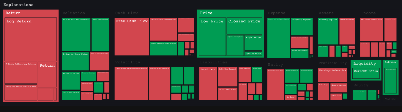
Feature Importance (Shapley Values) calculates the contribution of each input variable (features) such as Debt, Assets, and Revenue to predict bankruptcy risk.

<figure><img src="https://1304136543-files.gitbook.io/~/files/v0/b/gitbook-x-prod.appspot.com/o/spaces%2FCbqQ4ogM0YiEs5Z9Djdn%2Fuploads%2Fgit-blob-a182d0c74cb23990f87f244f86fdf352cc492d04%2Fbankruptcy_predictions_2.png?alt=media" alt=""><figcaption></figcaption></figure>

## Reports

### Sorting and Filtering

```python
import sovai as sov
sov.report("bankruptcy", report_type="ranking")
```

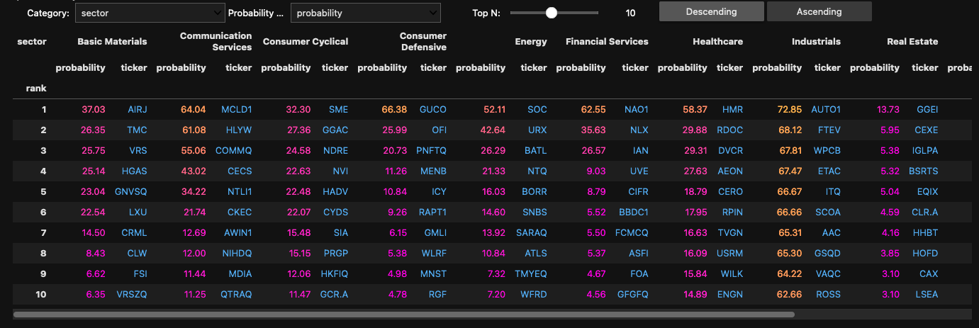
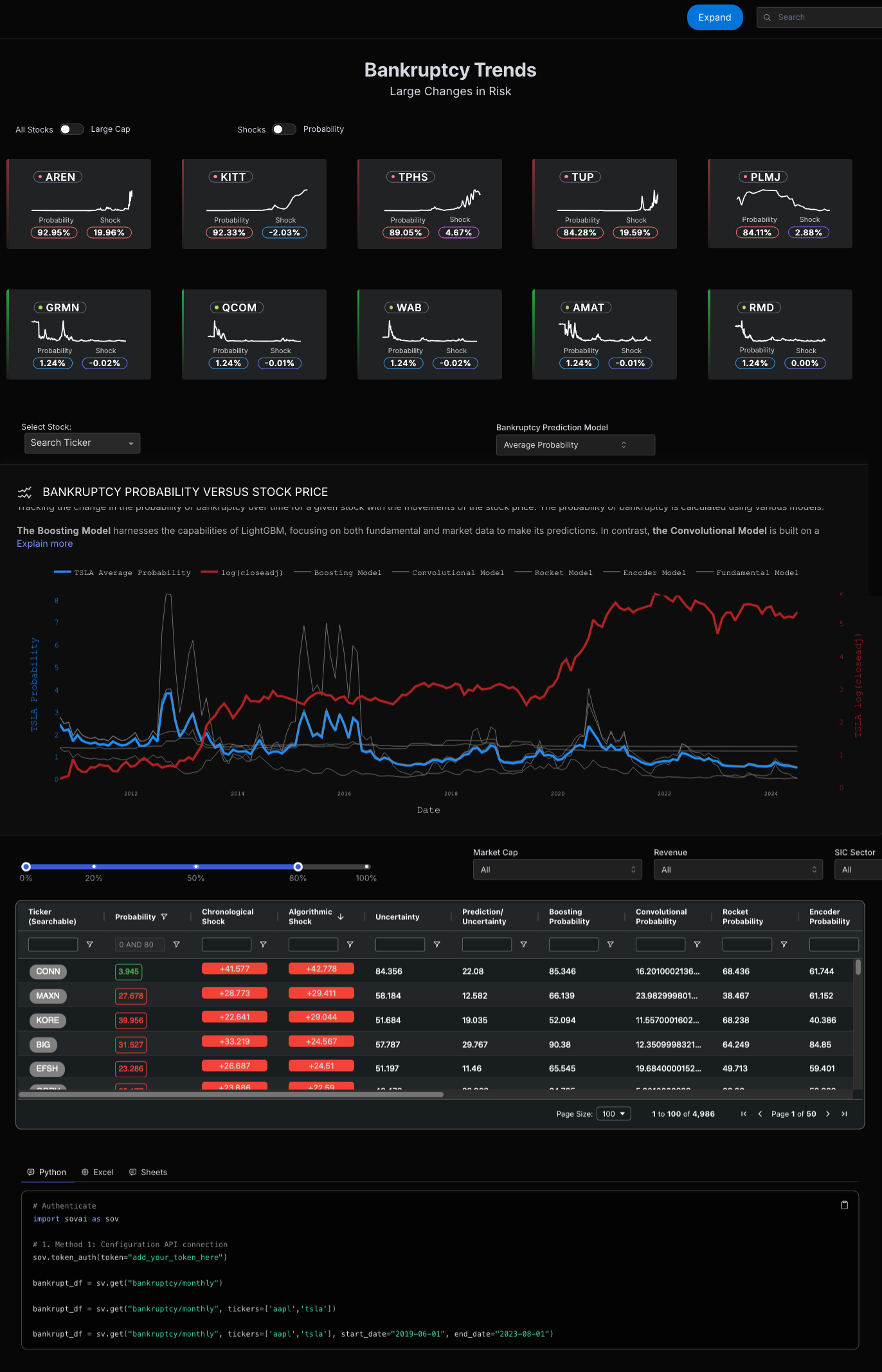
<figure><img src="https://1304136543-files.gitbook.io/~/files/v0/b/gitbook-x-prod.appspot.com/o/spaces%2FCbqQ4ogM0YiEs5Z9Djdn%2Fuploads%2Fgit-blob-1b040a5086bfa2c86458b649a204f2e28b11bd60%2Fbankruptcy_predictions_3.png?alt=media" alt=""><figcaption></figcaption></figure>

Filter the outputs based on the top by **Sector**, **Marketcap**, and **Revenue** and bankruptcy risk. You can also change <mark style="color:blue;">`ranking`</mark> to <mark style="color:blue;">`change`</mark> to investigate the month on month change.

```python
sov.report("bankruptcy", report_type="sector-change")
```

## Plots

### Bankruptcy Comparison

```python
import sovai as sov
sov.plot('bankruptcy', chart_type='compare')
```

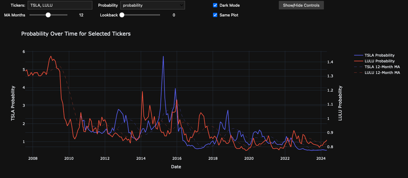
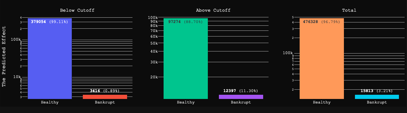
<figure><img src="https://1304136543-files.gitbook.io/~/files/v0/b/gitbook-x-prod.appspot.com/o/spaces%2FCbqQ4ogM0YiEs5Z9Djdn%2Fuploads%2Fgit-blob-354bd45745a52c9265dd751dfff92a7110188e5d%2Fbankruptcy_predictions_4.png?alt=media" alt=""><figcaption></figcaption></figure>

### Timed Feature Importance

```python
import sovai as sov
df = sov.plot("bankruptcy", chart_type="shapley", tickers=["TSLA"])
```

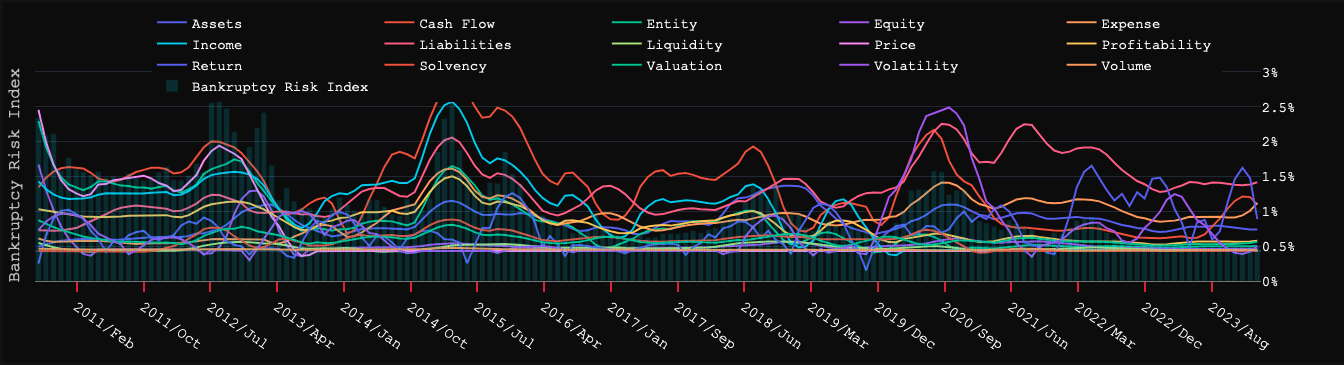
<figure><img src="https://1304136543-files.gitbook.io/~/files/v0/b/gitbook-x-prod.appspot.com/o/spaces%2FCbqQ4ogM0YiEs5Z9Djdn%2Fuploads%2Fgit-blob-02c13992eabf536dc4c9baa1acb3722b2e3bdfc7%2Fbankruptcy_predictions_5.png?alt=media" alt=""><figcaption></figcaption></figure>

### Total Feature Importance

```python
import sovai as sov
sov.plot("bankruptcy", chart_type="stack", tickers=["DDD"])
```

<figure><img src="https://1304136543-files.gitbook.io/~/files/v0/b/gitbook-x-prod.appspot.com/o/spaces%2FCbqQ4ogM0YiEs5Z9Djdn%2Fuploads%2Fgit-blob-9ba2eca3aff0c636d3af2f706c54ec6e8de2ef39%2Fbankruptcy_predictions_6.png?alt=media" alt=""><figcaption></figcaption></figure>

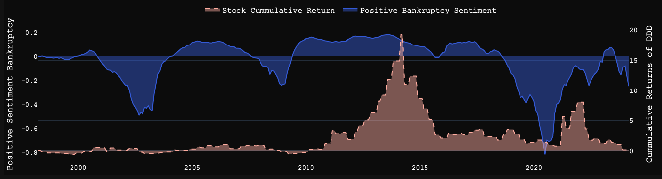
### Bankruptcy and Returns

```python
import sovai as sov
df= sov.plot("bankruptcy", chart_type="line", tickers=["DDD"])
```

<figure><img src="https://1304136543-files.gitbook.io/~/files/v0/b/gitbook-x-prod.appspot.com/o/spaces%2FCbqQ4ogM0YiEs5Z9Djdn%2Fuploads%2Fgit-blob-536df7450795c5ccce0089fa860102013b1ba5f7%2Fbankruptcy_predictions_7.png?alt=media" alt=""><figcaption></figcaption></figure>

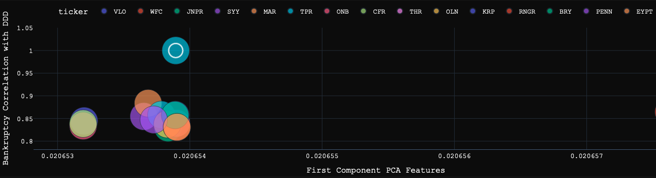
### **PCA Statistical Similarity**

```python
import sovai as sov
df= sov.plot("bankruptcy", chart_type="line", tickers=["DDD"])
```

<figure><img src="https://1304136543-files.gitbook.io/~/files/v0/b/gitbook-x-prod.appspot.com/o/spaces%2FCbqQ4ogM0YiEs5Z9Djdn%2Fuploads%2Fgit-blob-529d09c16609ea006ce09d313c8b04ce605dfb16%2Fbankruptcy_predictions_8.png?alt=media" alt=""><figcaption></figcaption></figure>

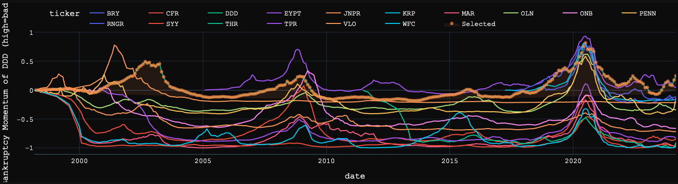
### Correlation Similarity

```python
import sovai as sov
sov.plot("bankruptcy", chart_type="similar", tickers=["DDD"])
```

<figure><img src="https://1304136543-files.gitbook.io/~/files/v0/b/gitbook-x-prod.appspot.com/o/spaces%2FCbqQ4ogM0YiEs5Z9Djdn%2Fuploads%2Fgit-blob-edb73ac63dcc6f2181a94442de34fc9ac4a00b81%2Fbankruptcy_predictions_9.png?alt=media" alt=""><figcaption></figcaption></figure>

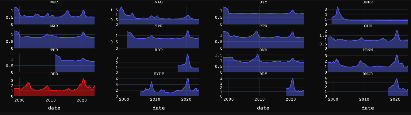
### Trend Similarity

```python
import sovai as sov
sov.plot("bankruptcy", chart_type="facet", tickers=["DDD"])
```

<figure><img src="https://1304136543-files.gitbook.io/~/files/v0/b/gitbook-x-prod.appspot.com/o/spaces%2FCbqQ4ogM0YiEs5Z9Djdn%2Fuploads%2Fgit-blob-bb6a98344aeca611bb2c7c1cc40f2f8cd5dbc32c%2Fbankruptcy_predictions_10.png?alt=media" alt=""><figcaption></figcaption></figure>

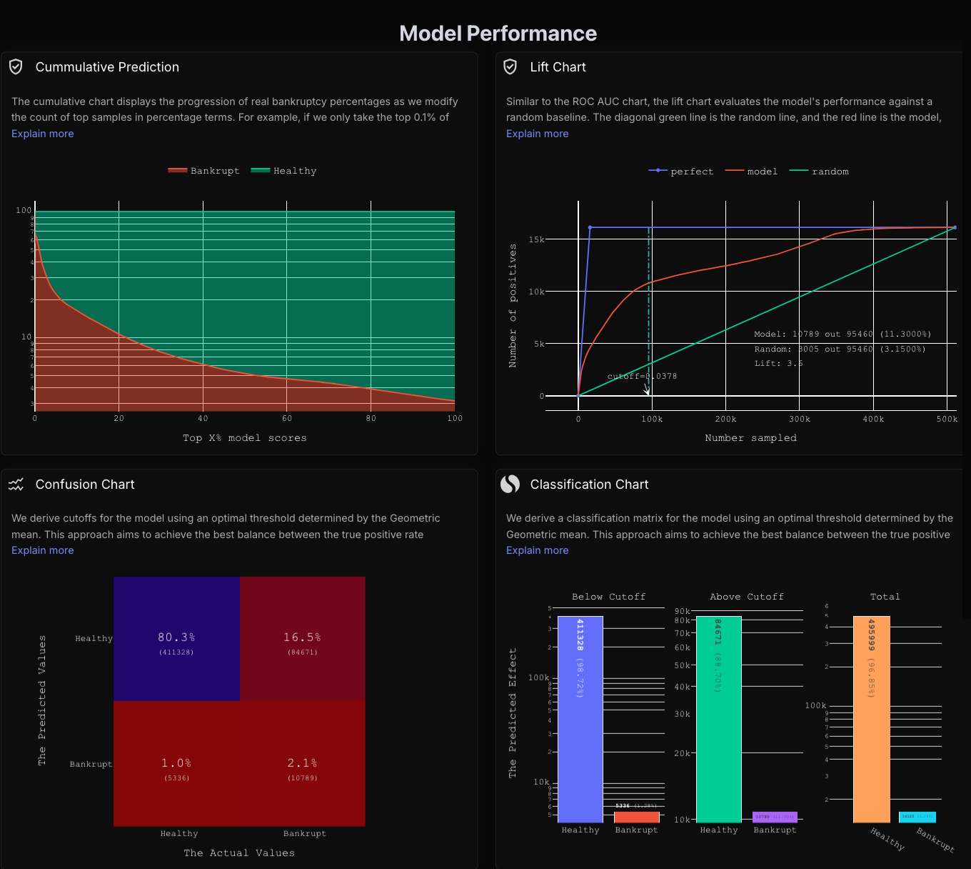
## Model Performance

### **Confusion Matrix**

```python
import sovai as sov
sov.plot("bankruptcy", chart_type="confusion_global")
```

<figure><img src="https://1304136543-files.gitbook.io/~/files/v0/b/gitbook-x-prod.appspot.com/o/spaces%2FCbqQ4ogM0YiEs5Z9Djdn%2Fuploads%2Fgit-blob-9abb9c10ac9b6681843a7985618dae646734d1e1%2Fbankruptcy_predictions_11.png?alt=media" alt=""><figcaption></figcaption></figure>

### **Threshold Plots**

```python
import sovai as sov
sov.plot("bankruptcy", chart_type="classification_global")
```

<figure><img src="https://1304136543-files.gitbook.io/~/files/v0/b/gitbook-x-prod.appspot.com/o/spaces%2FCbqQ4ogM0YiEs5Z9Djdn%2Fuploads%2Fgit-blob-43cc6dec6e269c515f6b51249d1d8672385c7c6b%2Fbankruptcy_predictions_12.png?alt=media" alt=""><figcaption></figcaption></figure>

### **Lift Curve**

```python
import sovai as sov
sov.plot("bankruptcy", chart_type="lift_global")
```

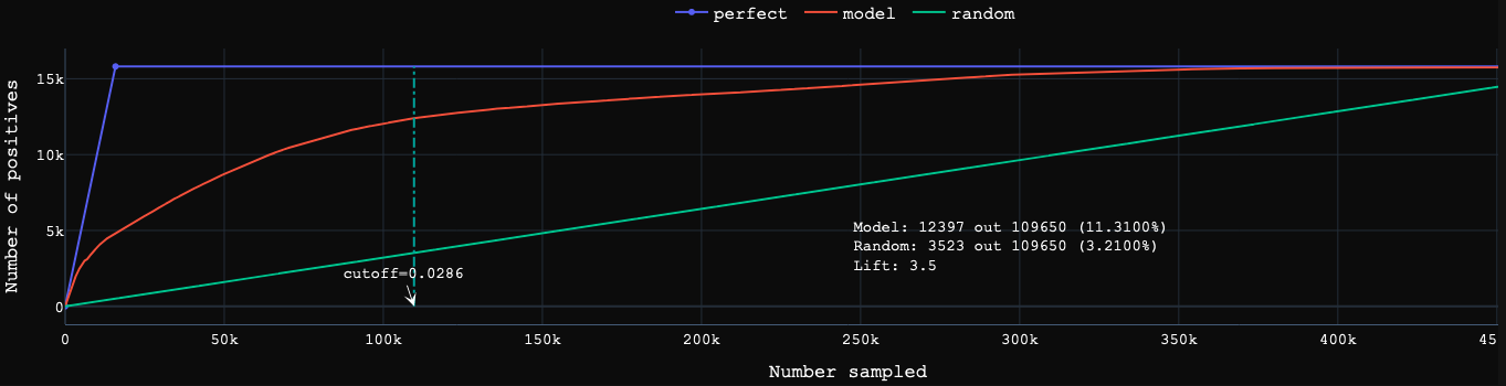
<figure><img src="https://1304136543-files.gitbook.io/~/files/v0/b/gitbook-x-prod.appspot.com/o/spaces%2FCbqQ4ogM0YiEs5Z9Djdn%2Fuploads%2Fgit-blob-72f9a2db7ad96ea07029500e14cb289dee227e1a%2Fbankruptcy_predictions_13.png?alt=media" alt=""><figcaption></figcaption></figure>

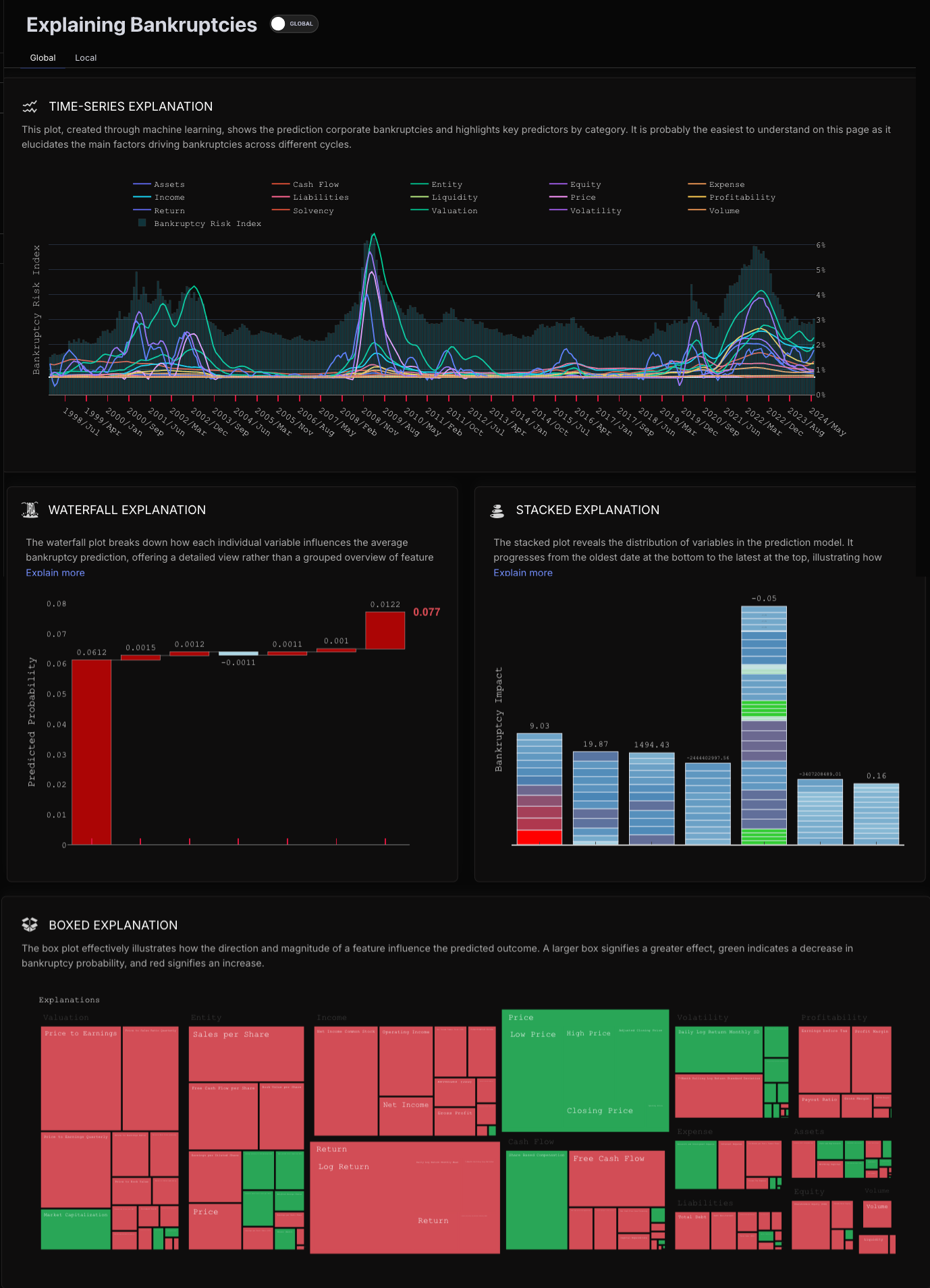
### Global Explainability

```python
import sovai as sov
sov.plot("bankruptcy", chart_type="time_global")
```

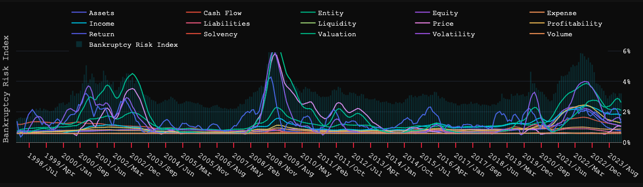
<figure><img src="https://1304136543-files.gitbook.io/~/files/v0/b/gitbook-x-prod.appspot.com/o/spaces%2FCbqQ4ogM0YiEs5Z9Djdn%2Fuploads%2Fgit-blob-1b0e786fa2ac21396740f4868ba85b55760a461f%2Fbankruptcy_predictions_14.png?alt=media" alt=""><figcaption></figcaption></figure>

## Computations

Leverage advanced computational tools for deeper analysis:

* **Distance Matrix:**

  ```python
  sov.compute('distance-matrix', on="attribute", df=dataframe)
  ```

  Assess the similarity between entities based on selected attributes.
* **Percentile Calculation:**

  ```python
  sov.compute('percentile', on="attribute", df=dataframe)
  ```

  Calculate the relative standing of values within a dataset.
* **Feature Mapping:**

  ```python
  sov.compute('map-accounting-features', df=dataframe)
  ```

  Map accounting features to standardized metrics.
* **PCA Calculation:**

  ```python
  sov.compute('pca', df=dataframe)
  ```

  Perform principal component analysis for dimensionality reduction.

**For more advanced applications, see the tutotrial.**

## Data Dictionary

<table><thead><tr><th width="293">Name</th><th width="246">Description</th><th width="89">Type</th><th>Example</th></tr></thead><tbody><tr><td><code>ticker</code></td><td>Stock ticker symbol.</td><td>TEXT</td><td>"TSLA"</td></tr><tr><td><code>date</code></td><td>Record date.</td><td>DATE</td><td>2023-09-30</td></tr><tr><td><code>probability_light</code></td><td>LightGBM Boosting Model prediction.</td><td>FLOAT</td><td>1.46636</td></tr><tr><td><code>probability_convolution</code></td><td>CNN Model prediction for bankruptcies</td><td>FLOAT</td><td>0.135975</td></tr><tr><td><code>probability_rocket</code></td><td>Rocket Model prediction for time series classification</td><td>FLOAT</td><td>0.02514</td></tr><tr><td><code>probability_encoder</code></td><td>LightGBM and CNN autoencoders Model prediction.</td><td>FLOAT</td><td>0.587817</td></tr><tr><td><code>probability_fundamental</code></td><td>Prediction using accounting data only.</td><td>FLOAT</td><td>1.26148</td></tr><tr><td><code>probability</code></td><td>Average probability across models.</td><td>FLOAT</td><td>0.553823</td></tr><tr><td><code>sans_market</code></td><td>Fundamental prediction adjusted for market predictions.</td><td>FLOAT</td><td>-0.20488</td></tr><tr><td><code>volatility</code></td><td>Variability of model predictions.</td><td>FLOAT</td><td>0.62934</td></tr><tr><td><code>multiplier</code></td><td>Coefficient for model prediction calibration.</td><td>FLOAT</td><td>1.951868</td></tr><tr><td><code>version</code></td><td>Model/data record version.</td><td>INT</td><td>20240201</td></tr></tbody></table>

{% hint style="info" %}
When `sans_market` is <mark style="color:green;">positive</mark>, it means that the fundamentals show a larger predicted bankruptcy than what the market predicts **(stock might go down in medium term)** , when `sans_market` is <mark style="color:red;">negative</mark>, the market might have overreacted, and predict a larger probability of bankruptcy than what the fundamentals suggest **(stock might go up in medium term)**.
{% endhint %}

## Use Cases

1. **Bankruptcy Prediction Analysis**: Offer insights into predicted corporate bankruptcies and identify key factors, clarifying main drivers across different cycles.
2. **Variable Impact Breakdown**: Analyze how each individual variable affects bankruptcy predictions, providing in-depth feature contribution insights.
3. **Temporal Feature Distribution Analysis**: Reveal how variables contribute to predictions over time, emphasizing key features in forecasting models.
4. **Correlation Discovery**: Identify stocks with similar bankruptcy probability trends, revealing correlated market behaviors.
5. **Probability Shift Overview**: Showcase changes in bankruptcy probabilities among correlated stocks, providing a comprehensive market perspective.
6. **Sentiment Inversion Analysis**: Convert bankruptcy predictions into positive sentiment indicators to gauge potential impacts on stock returns.
7. **Behavioral Similarity Mapping**: Locate stocks with similar behaviors to a selected reference, based on bankruptcy trends and PCA feature analysis.


# Employee Visa

The H1B dataset offers quarterly insights into foreign hiring trends, job details, and wages for informed decision-making.

{% hint style="info" %}
Data arrives late Friday night 11 pm - 12 as new **quarterly data** becomes available.
{% endhint %}

{% hint style="success" %}
Dataset contains 2500+ tickers, available from 2009-05-01 onwards.
{% endhint %}

`Tutorials` are the best documentation — [<mark style="color:blue;">`Employee Visa Tutorial`</mark>](https://colab.research.google.com/github/sovai-research/sovai-public/blob/main/notebooks/datasets/Employee%20Visa.ipynb)

<table data-column-title-hidden data-view="cards"><thead><tr><th>Category</th><th>Details</th></tr></thead><tbody><tr><td><strong>Input Datasets</strong></td><td>Government Data</td></tr><tr><td><strong>Models Used</strong></td><td>Parsing, Regex</td></tr><tr><td><strong>Model Outputs</strong></td><td>Standardized Rows</td></tr></tbody></table>

## Description

The Employee Visa dataset provides quarterly insights into foreign hiring trends among U.S. companies, offering detailed information on job positions, wages, and visa applications across various temporary work visa categories.

This data can serve as a valuable tool for investors to analyze labor market trends, assess company growth strategies, and gauge the impact of immigration policies on different sectors and businesses.

## Data Access

**H1B Table**: This table offers quarterly data to track foreign hiring patterns for publicly traded companies.

```python
import sovai as sov
df_visa = sov.data("visas/h1b", start_date="2010-01-01", tickers=["MSFT","TSLA"])
```

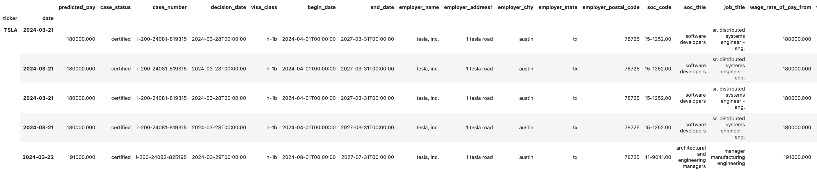
<figure><img src="https://1304136543-files.gitbook.io/~/files/v0/b/gitbook-x-prod.appspot.com/o/spaces%2FCbqQ4ogM0YiEs5Z9Djdn%2Fuploads%2Fgit-blob-ab5f011de2db74ee340d78cd3a1581913df1e608%2Femployee_visa_1.png?alt=media" alt=""><figcaption></figcaption></figure>

This dataset encompasses detailed records from labor condition applications, which are indicative of employment patterns within companies that hire foreign workers under various temporary visa categories in the United States. It provides a comprehensive view of job positions, wages, and employment periods.

## Data Dictionary

<table><thead><tr><th width="198">Name</th><th width="314">Description</th><th width="114">Type</th><th>Example</th></tr></thead><tbody><tr><td>predicted_pay</td><td>Predicted salary for the job position</td><td>float64</td><td>190195</td></tr><tr><td>case_status</td><td>Status of the case/application</td><td>object</td><td>certified</td></tr><tr><td>case_number</td><td>Unique identifier for the case/application</td><td>object</td><td>i-203-17089-869756</td></tr><tr><td>decision_date</td><td>Date on which the decision was made</td><td>object</td><td>2017-04-06 0:00:00</td></tr><tr><td>visa_class</td><td>Type of visa applied for</td><td>object</td><td>e-3 australian</td></tr><tr><td>begin_date</td><td>Start date of employment</td><td>object</td><td>2017-07-02 0:00:00</td></tr><tr><td>end_date</td><td>End date of employment</td><td>object</td><td>2019-07-01 0:00:00</td></tr><tr><td>employer_name</td><td>Name of the employer</td><td>object</td><td>apple inc.</td></tr><tr><td>employer_address1</td><td>Address line of the employer</td><td>object</td><td>one infinite loop</td></tr><tr><td>employer_city</td><td>City where the employer is located</td><td>object</td><td>cupertino</td></tr><tr><td>employer_state</td><td>State where the employer is located</td><td>object</td><td>ca</td></tr><tr><td>employer_postal_code</td><td>Postal code of the employer</td><td>object</td><td>95014</td></tr><tr><td>soc_code</td><td>Standard Occupational Classification code</td><td>object</td><td>11-3021</td></tr><tr><td>soc_title</td><td>Title associated with the SOC code</td><td>object</td><td>computer and information systems managers</td></tr><tr><td>job_title</td><td>Title of the job</td><td>object</td><td>sw develop mgr 3</td></tr><tr><td>wage_rate_of_pay_from</td><td>Starting wage rate</td><td>float64</td><td>190195</td></tr><tr><td>wage_rate_of_pay_to</td><td>Ending wage rate</td><td>float64</td><td>190195</td></tr><tr><td>wage_unit_of_pay</td><td>Unit for the wage rate</td><td>object</td><td>year</td></tr><tr><td>full_time_position</td><td>Whether the position is full-time</td><td>object</td><td>y</td></tr><tr><td>worksite_address2</td><td>Secondary worksite address</td><td>object</td><td>None</td></tr><tr><td>worksite_state</td><td>State of the worksite</td><td>object</td><td>ca</td></tr><tr><td>prevailing_wage</td><td>Standard wage for the position</td><td>float64</td><td>190195</td></tr><tr><td>pw_unit_of_pay</td><td>Unit for the prevailing wage</td><td>object</td><td>year</td></tr><tr><td>pw_survey_name</td><td>Name of the prevailing wage survey</td><td>object</td><td>None</td></tr><tr><td>pw_other_source</td><td>Other source for prevailing wage</td><td>object</td><td>oflc online data center</td></tr><tr><td>pw_oes_year</td><td>Year of the OES prevailing wage</td><td>float64</td><td>2016</td></tr><tr><td>pw_survey_publisher</td><td>Publisher of the prevailing wage survey</td><td>object</td><td>None</td></tr><tr><td>naics_code</td><td>North American Industry Classification System code</td><td>float64</td><td>334111</td></tr><tr><td>unique_id</td><td>Unique identifier combining case number, soc_code, and employer state</td><td>object</td><td>i-203-17089-869756_11-3021_ca</td></tr><tr><td>wage_potential_increase</td><td>Potential increase in wage</td><td>float64</td><td>0</td></tr><tr><td>similarity</td><td>Similarity score</td><td>float64</td><td>1</td></tr><tr><td>bloomberg_share_id</td><td>Bloomberg's share identifier</td><td>object</td><td>BBG001S5N8V8</td></tr><tr><td>total_worker_positions</td><td>Total number of worker positions</td><td>float64</td><td>1</td></tr><tr><td>new_employment</td><td>Indicates new employment</td><td>float64</td><td>0</td></tr><tr><td>continued_employment</td><td>Indicates continued employment</td><td>float64</td><td>1</td></tr><tr><td>change_previous_employment</td><td>Indicates a change in previous employment</td><td>float64</td><td>0</td></tr><tr><td>new_concurrent_employment</td><td>Indicates new concurrent employment</td><td>float64</td><td>0</td></tr><tr><td>change_employer</td><td>Indicates a change of employer</td><td>float64</td><td>0</td></tr><tr><td>amended_petition</td><td>Indicates if there is an amended petition</td><td>float64</td><td>0</td></tr></tbody></table>

The dataset includes 39 columns, each representing a specific attribute related to labor condition applications. Key attributes include:

* Case status and number, providing insight into the application's outcome and unique identification.
* Visa class, which distinguishes between different types of temporary work visas.
* Employment period, outlined by the begin and end dates of employment.
* Employer information, including name, address, city, state, and postal code.
* Job details, such as job title, Standard Occupational Classification (SOC) code and title.
* Wage information, including the rate of pay and prevailing wage details.
* Worksite information, offering location details where the employment takes place.
* Additional attributes related to the petition's nature, like new employment, continued employment, and any amendments.

***

## Use Cases

1. **Labor Market Analysis**: Investors can identify trends in employment such as demand for specific roles or average wages offered across sectors, informing investment strategies.
2. **Compliance Monitoring**: Companies can ensure their wage offerings are competitive and compliant with prevailing wage standards for different visa categories.
3. **Immigration Impact Assessment**: Policy analysts can evaluate the effects of visa policies on workforce composition and availability in various industries.
4. **Strategic Planning**: Businesses can plan recruitment strategies based on the availability of talent within certain visa classes and adjust their workforce accordingly.
5. **Investment Decision Making**: Investors can gauge the health and growth potential of sectors by analyzing the number of new and continuing employment positions.

***


# Earnings Surprise

Earnings announcements are obtained from external sources as well as estimate information leading up to the actual announcement.

{% hint style="info" %}
Data arrives late Friday night 11 pm - 12; the model also retrains weekly.
{% endhint %}

{% hint style="success" %}
Dataset contains 4330+ tickers, available from 2016-12-30 onwards.
{% endhint %}

`Tutorials` are the best documentation — [<mark style="color:blue;">`Earnings Surprise Tutorial`</mark>](https://colab.research.google.com/github/sovai-research/sovai-public/blob/main/notebooks/datasets/Earnings%20Surprise.ipynb)

<table data-column-title-hidden data-view="cards"><thead><tr><th>Category</th><th>Details</th></tr></thead><tbody><tr><td><strong>Input Datasets</strong></td><td>Public filings, news, analyst reports</td></tr><tr><td><strong>Models Used</strong></td><td>Parsing, Regex</td></tr><tr><td><strong>Model Outputs</strong></td><td>Standardized Rows</td></tr></tbody></table>

## Description

The **Earnings Surprise** dataset provides detailed insights into the financial performance of publicly traded companies by capturing the discrepancies between reported earnings and analysts' estimates. This dataset includes metrics such as the probability of an earnings surprise, the magnitude of earnings per share (EPS) surprises, actual earnings results, estimated earnings, and the publication dates of earnings reports.

By offering a granular view of earnings performance, this data serves as a vital tool for investors to assess company performance, predict stock price movements, and make informed investment decisions based on the reliability and accuracy of earnings forecasts.

## Data Access

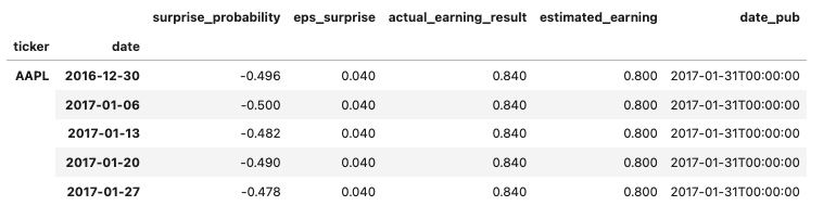
```python
import sovai as sov
df_earn_surp = sov.data("earnings/surprise", tickers=["AAPL", "MSFT"])
```

<figure><img src="https://1304136543-files.gitbook.io/~/files/v0/b/gitbook-x-prod.appspot.com/o/spaces%2FCbqQ4ogM0YiEs5Z9Djdn%2Fuploads%2Fgit-blob-0ee5623bed9d69f796d906725aab2cd75d3bd512%2Fearnings_surprise_1.png?alt=media" alt=""><figcaption></figcaption></figure>

## Data Dictionary

| **Name**                | **Description**                               | **Type** | **Example**           |
| ----------------------- | --------------------------------------------- | -------- | --------------------- |
| `ticker`                | Stock ticker symbol of the company            | object   | `AAPL`                |
| `date`                  | Date of the earnings report                   | object   | `2016-12-30`          |
| `surprise_probability`  | Probability of an earnings surprise occurring | float64  | `-0.496`              |
| `eps_surprise`          | Earnings per share surprise value             | float64  | `0.040`               |
| `actual_earning_result` | Actual reported earnings per share            | float64  | `0.840`               |
| `estimated_earning`     | Analysts' estimated earnings per share        | float64  | `0.800`               |
| `date_pub`              | Publication date of the earnings report       | object   | `2017-01-31T00:00:00` |
| `market_cap`            | Market capitalization of the company (in USD) | float64  | `1.5e+12`             |

***

## Use Cases

* **Investment Signal Generation:** Utilize earnings surprise metrics to identify potential investment opportunities by spotting companies that consistently outperform or underperform earnings expectations.
* **Risk Management:** Assess the risk associated with investments by monitoring the frequency and magnitude of earnings surprises, identifying companies with unstable earnings.
* **Event-Driven Investment Strategies:** Develop strategies around earnings report dates, capitalizing on anticipated surprises to execute buy or sell orders based on expected market reactions.

***


# Congressional Data

From filings we collect and match trades in the Senate and House and make them available within a day of processing.

{% hint style="info" %}
Data arrives daily or as new trades are being made triggering the processing of the data.
{% endhint %}

{% hint style="success" %}
Dataset contains 4000+ tickers, available from 2014-03-01 onwards.
{% endhint %}

`Tutorials` are the best documentation — [<mark style="color:blue;">`Congressional Tutorial`</mark>](https://colab.research.google.com/github/sovai-research/sovai-public/blob/main/notebooks/datasets/Congressional%20Trading.ipynb)

<table data-column-title-hidden data-view="cards"><thead><tr><th>Category</th><th>Details</th></tr></thead><tbody><tr><td><strong>Input Datasets</strong></td><td>House and Senator Filings</td></tr><tr><td><strong>Models Used</strong></td><td>Parsing, Regex</td></tr><tr><td><strong>Model Outputs</strong></td><td>Standardized Rows</td></tr></tbody></table>

## Description

The Congressional Trading dataset offers comprehensive insights into the financial transactions of U.S. Congress members, encompassing both Senate and House representatives. This dataset includes detailed information on securities traded, transaction dates, types of transactions (e.g., purchases, sales), transaction amounts, political party affiliations, and pertinent biographical details of each legislator.

By providing transparency into the investment activities of elected officials, this data serves as a crucial tool for constituents, analysts, investors, and policymakers to monitor potential conflicts of interest, assess ethical compliance, and understand the financial behaviors of those in power.

## Data Access

The easiest is to just download the dump and to filter data from there, this is updated on a daily basis.

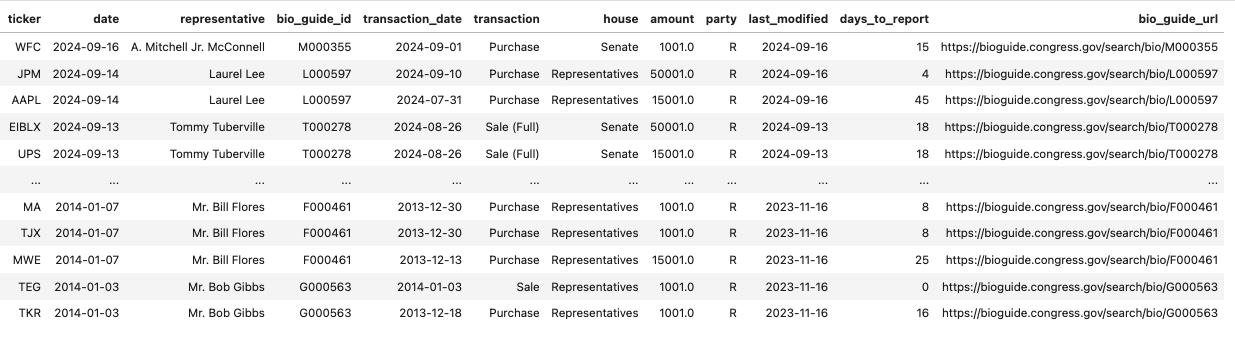
```python
import sovai as sov
df_congress = sov.data("congress")
```

<figure><img src="https://1304136543-files.gitbook.io/~/files/v0/b/gitbook-x-prod.appspot.com/o/spaces%2FCbqQ4ogM0YiEs5Z9Djdn%2Fuploads%2Fgit-blob-854a67616b1107bf56fd0e5c0aa951cd4dd1fdc8%2Fcongressional_data_1.png?alt=media" alt=""><figcaption></figcaption></figure>

## Data Dictionary

| **Name**           | **Description**                                   | **Type** | **Example**                                        |
| ------------------ | ------------------------------------------------- | -------- | -------------------------------------------------- |
| `ticker`           | Stock ticker symbol traded by the representative  | object   | `AAPL`                                             |
| `date`             | Date the transaction was reported                 | object   | `2024-09-16`                                       |
| `representative`   | Name of the congressional representative          | object   | `A. Mitchell Jr. McConnell`                        |
| `bio_guide_id`     | Biographical identifier for the representative    | object   | `M000355`                                          |
| `transaction_date` | Date when the transaction occurred                | object   | `2024-09-01`                                       |
| `transaction`      | Type of transaction (e.g., Purchase, Sale)        | object   | `Purchase`                                         |
| `house`            | Congressional house affiliation (Senate or House) | object   | `Senate`                                           |
| `amount`           | Amount of the transaction in USD                  | float64  | `1001.0`                                           |
| `party`            | Political party affiliation of the representative | object   | `R` (Republican)                                   |
| `last_modified`    | Date the record was last updated                  | object   | `2024-09-16`                                       |
| `days_to_report`   | Number of days taken to report the transaction    | int64    | `15`                                               |
| `bio_guide_url`    | URL to the representative's biographical page     | object   | `https://bioguide.congress.gov/search/bio/M000355` |

***

***

## Use Cases

1. Investment Signal Generation: Utilize trading activities of congressional members to identify potential investment opportunities and market trends.
2. Insider Trading Detection: Monitor transactions by lawmakers to spot unusual trading patterns that may indicate insider information usage.
3. Sector Influence Analysis: Analyze which sectors are frequently traded by representatives to anticipate legislative support and its impact on those industries.
4. Portfolio Diversification: Incorporate insights from congressional trading data to diversify investments based on the financial behaviors of elected officials.

***


# Factor Signals

A financial factor dataset for in-depth company analysis and investment strategies.

{% hint style="info" %}
Data is updated weekly as data arrives after market close US-EST time.
{% endhint %}

{% hint style="success" %}
Dataset contains 6400+ tickers, available from 1998-01-09 onwards.
{% endhint %}

`Tutorials` are the best documentation — [<mark style="color:blue;">`Factor Signals Tutorial`</mark>](https://colab.research.google.com/github/sovai-research/sovai-public/blob/main/notebooks/datasets/Factor%20Model.ipynb)

<table data-column-title-hidden data-view="cards"><thead><tr><th>Category</th><th>Details</th></tr></thead><tbody><tr><td><strong>Input Datasets</strong></td><td>Filings, Financial Data</td></tr><tr><td><strong>Models Used</strong></td><td>OLS Regression</td></tr><tr><td><strong>Model Outputs</strong></td><td>Factors, Coefficients, Standard Errors</td></tr></tbody></table>

## Description

This dataset includes traditional accounting factors, alternative financial metrics, and advanced statistical analyses, enabling sophisticated financial modeling.

It could be used for bottom-up equity selection strategies and for the development of investment strategies.

***

## Data Access

#### Comprehensive Factors

Comprehensive Factors dataset is a merged set of both accounting and alternative financial metrics, providing a holistic view of a company's financial status.

```python
import sovai as sov
df_factor_comp = sov.data("factors/comprehensive",tickers=["MSFT","TSLA"])
```

<figure><img src="https://1304136543-files.gitbook.io/~/files/v0/b/gitbook-x-prod.appspot.com/o/spaces%2FCbqQ4ogM0YiEs5Z9Djdn%2Fuploads%2Fgit-blob-73329b305a415d825702cc0735af6246d6f18416%2Ffactor_signals_1.png?alt=media" alt=""><figcaption></figcaption></figure>

#### Accounting Factors

The Accounting Factors dataset includes key financial metrics related to accounting for various companies.

```python
import sovai as sov
df_factor_actn = sov.data("factors/accounting",tickers=["MSFT","TSLA"])
```

#### Alternative Factors

This dataset contains alternative financial factors that are not typically found in standard financial statements.

```python
import sovai as sov
df_factor_alt = sov.data("factors/alternative",tickers=["MSFT","TSLA"])
```

#### Coefficients Factors

The Coefficients Factors dataset includes various coefficients related to different financial metrics.

<pre class="language-python"><code class="lang-python">import sovai as sov
<strong>df_factor_coeff = sov.data("factors/coefficients",tickers=["MSFT","TSLA"])
</strong></code></pre>

#### Standard Errors Factors

This dataset provides standard errors for various financial metrics, useful for statistical analysis and modeling.

```python
import sovai as sov
df_factor_std_err = get_data("factors/standard_errors",tickers=["MSFT","TSLA"])
```

#### T-Statistics Factors

The T-Statistics Factors dataset includes t-statistics for different financial metrics, offering insights into their significance.

```python
import sovai as sov
df_factor_t_stat = get_data("factors/t_statistics",tickers=["MSFT","TSLA"])
```

#### Model Metrics

Model Metrics dataset includes various metrics such as R-squared, AIC, BIC, etc., that are crucial for evaluating the performance of financial models.

```python
import sovai as sov
df_model_metrics = sov.data("factors/model_metrics",tickers=["MSFT","TSLA"])
```

***

This documentation provides a clear guide on how to access each dataset, and can be easily extended or modified as needed for additional datasets or details.

## Data Dictionary

### Financial Factors Dataset

<table><thead><tr><th width="286">Name</th><th>Description</th></tr></thead><tbody><tr><td><code>ticker</code></td><td>The unique identifier for a publicly traded company's stock.</td></tr><tr><td><code>date</code></td><td>The specific date for which the data is recorded.</td></tr><tr><td><code>profitability</code></td><td>A measure of a company's efficiency in generating profits.</td></tr><tr><td><code>value</code></td><td>Indicates the company's market value, often reflecting its perceived worth.</td></tr><tr><td><code>solvency</code></td><td>Reflects the company's ability to meet its long-term financial obligations.</td></tr><tr><td><code>cash_flow</code></td><td>Represents the amount of cash being transferred into and out of a business.</td></tr><tr><td><code>illiquidity</code></td><td>Measures the difficulty of converting assets into cash quickly without significant loss in value.</td></tr><tr><td><code>momentum_long_term</code></td><td>Indicates long-term trends in the company's stock price movements.</td></tr><tr><td><code>momentum_medium_term</code></td><td>Represents medium-term trends in stock price movements.</td></tr><tr><td><code>short_term_reversal</code></td><td>Reflects short-term price reversals in the stock market.</td></tr><tr><td><code>price_volatility</code></td><td>Measures the degree of variation in a company's stock price over time.</td></tr><tr><td><code>dividend_yield</code></td><td>The dividend per share, divided by the price per share, showing how much a company pays out in dividends each year relative to its stock price.</td></tr><tr><td><code>earnings_consistency</code></td><td>Indicates the stability and predictability of a company's earnings over time.</td></tr><tr><td><code>small_size</code></td><td>A factor indicating the company's size, with smaller companies potentially offering higher returns (albeit with higher risk).</td></tr><tr><td><code>low_growth</code></td><td>Reflects the company's lower-than-average growth prospects.</td></tr><tr><td><code>low_equity_issuance</code></td><td>Indicates a lower level of issuing new shares, which can be a sign of financial strength or limited growth prospects.</td></tr><tr><td><code>bounce_dip</code></td><td>Measures the tendency of a stock to recover quickly after a significant drop.</td></tr><tr><td><code>accrual_growth</code></td><td>Represents the growth rate in accruals, which are earnings not yet realized in cash.</td></tr><tr><td><code>low_depreciation_growth</code></td><td>Indicates lower growth in depreciation expenses, which might suggest more stable capital expenditures.</td></tr><tr><td><code>current_liquidity</code></td><td>A measure of a company's ability to pay off its short-term liabilities with its short-term assets.</td></tr><tr><td><code>low_rnd</code></td><td>Reflects lower expenditures on research and development, which could indicate less investment in future growth.</td></tr><tr><td><code>momentum</code></td><td>Overall momentum factor, representing the general trend in the stock price movements.</td></tr><tr><td><code>market_risk</code></td><td>Indicates the risk of an investment in a particular market relative to the entire market.</td></tr><tr><td><code>business_risk</code></td><td>Reflects the inherent risk associated with the specific business activities of a company.</td></tr><tr><td><code>political_risk</code></td><td>Measures the potential for losses due to political instability or changes in a country's political environment.</td></tr><tr><td><code>inflation_fluctuation</code></td><td>Indicates how sensitive the company is to fluctuations in inflation rates.</td></tr><tr><td><code>inflation_persistence</code></td><td>Measures the company's exposure to persistent inflation trends.</td></tr><tr><td><code>returns</code></td><td>Represents the financial returns generated by the company over a specified period.</td></tr></tbody></table>

### ModelMetrics Dataset

<table><thead><tr><th width="267">Name</th><th>Description</th></tr></thead><tbody><tr><td><code>ticker</code></td><td>The unique stock ticker symbol identifying the company.</td></tr><tr><td><code>date</code></td><td>The date for which the model metrics are calculated.</td></tr><tr><td><code>rsquared</code></td><td>The R-squared value, indicating the proportion of variance in the dependent variable that's predictable from the independent variables.</td></tr><tr><td><code>rsquared_adj</code></td><td>The adjusted R-squared value, accounting for the number of predictors in the model (provides a more accurate measure when dealing with multiple predictors).</td></tr><tr><td><code>fvalue</code></td><td>The F-statistic value, used to determine if the overall regression model is a good fit for the data.</td></tr><tr><td><code>aic</code></td><td>Akaike’s Information Criterion, a measure of the relative quality of statistical models for a given set of data. Lower AIC indicates a better model.</td></tr><tr><td><code>bic</code></td><td>Bayesian Information Criterion, similar to AIC but with a higher penalty for models with more parameters.</td></tr><tr><td><code>mse_resid</code></td><td>Mean Squared Error of the residuals, measuring the average of the squares of the errors, i.e., the average squared difference between the estimated values and the actual value.</td></tr><tr><td><code>mse_total</code></td><td>Total Mean Squared Error, measuring the total variance in the observed data.</td></tr></tbody></table>

In addition to the primary financial metrics and model metrics, our data suite includes three specialized datasets:

* **Coefficients**: This dataset provides regression coefficients for various financial factors. These coefficients offer insights into the relative importance and impact of each factor in financial models.
* **Standard Errors**: Accompanying the coefficients, this dataset provides the standard error for each coefficient. The standard errors are crucial for understanding the precision and reliability of the coefficients in the model.
* **T-Statistics**: This dataset contains the t-statistic for each coefficient, a key metric for determining the statistical significance of each financial factor. It helps in evaluating the robustness of the coefficients' impact in the model.

These datasets form a comprehensive toolkit for financial analysis, enabling detailed regression analysis and statistical evaluation of financial factors.

### Factor Analysis Datasets

Our suite of Factor Analysis datasets offers a rich and comprehensive resource for investors seeking to deepen their understanding of market dynamics and enhance their investment strategies. Here's an overview of each dataset and its potential use cases:

#### Comprehensive Financial Metrics

1. **Accounting Factors (`FactorsAccounting`)**: This dataset includes core financial metrics like profitability, solvency, and cash flow. It's invaluable for fundamental analysis, enabling investors to assess a company's financial health and operational efficiency.
2. **Alternative Factors (`FactorsAlternative`)**: Focusing on non-traditional financial metrics such as market risk, business risk, and political risk, this dataset helps in evaluating external factors that could impact a company's performance.
3. **Comprehensive Factors (`FactorsComprehensive`)**: A merged set of accounting and alternative factors providing a holistic view of a company's status. This dataset is perfect for a comprehensive financial analysis, blending traditional and modern financial metrics.

#### Advanced Statistical Analysis

1. **Coefficients (`FactorsCoefficients`)**: Reveals the weight or importance of each financial factor in a statistical model. Investors can use this to identify which factors are most influential in predicting stock performance.
2. **Standard Errors (`FactorsStandardErrors`)**: Provides precision levels of the coefficients. This is crucial for investors in assessing the reliability of the coefficients in predictive models.
3. **T-Statistics (`FactorsTStatistics`)**: Offers insights into the statistical significance of each factor. Investors can use this to gauge the robustness and credibility of the factors in their investment models.
4. **Model Metrics (`ModelMetrics`)**: Includes advanced metrics like R-squared, AIC, and BIC. This dataset is essential for evaluating the effectiveness of financial models, helping investors to choose the most reliable models for their investment decisions.

#### Potential Use Cases

* **Portfolio Construction and Optimization**: By understanding the importance and impact of various financial factors, investors can construct and optimize their portfolios to maximize returns and minimize risks.
* **Risk Assessment and Management**: Alternative factors, along with risk-related metrics from other datasets, enable investors to conduct thorough risk assessments, leading to better risk management strategies.
* **Market Trend Analysis**: Long-term and medium-term momentum factors can be used for identifying prevailing market trends, aiding in strategic investment decisions.
* **Statistical Model Validation**: Investors can validate their financial models using model metrics and statistical datasets (Standard Errors and T-Statistics), ensuring robustness and reliability in their analysis.

###

***


# Financial Ratios

More than 80+ financial ratios calculated from financial statement and market data.

{% hint style="warning" %}
This dataset is replaceable with your preferred standardized ratio dataset, currently it is built from public filings with the values 95% confirmed against five commercial datasets.
{% endhint %}

{% hint style="info" %}
Data arrives late Friday night 11 pm - 12 am after market close US-EST time.
{% endhint %}

{% hint style="success" %}
Dataset contains 6400+ tickers, available from 1998-01-02 onwards.
{% endhint %}

`Tutorials` are the best documentation — [<mark style="color:blue;">`Financial Ratio Analyis Tutorial`</mark>](https://colab.research.google.com/github/sovai-research/sovai-public/blob/main/notebooks/datasets/Financial%20Ratios.ipynb)

<table data-column-title-hidden data-view="cards"><thead><tr><th>Category</th><th>Details</th></tr></thead><tbody><tr><td><strong>Input Datasets</strong></td><td>SEC Filings, EDGAR API, Exchange Data.</td></tr><tr><td><strong>Models Used</strong></td><td>Transformations, Simple Maths</td></tr><tr><td><strong>Model Outputs</strong></td><td>Standardized Ratios</td></tr></tbody></table>

## Description

Diversified selection of ratios for factor development or bottom-up equity selection strategies. The Financial Ratios dataset offers over 80 standardized financial ratios calculated from financial statements and market data, updated weekly after market close.

This comprehensive set of ratios, covering categories such as liquidity, profitability, efficiency, solvency, cash flow, and valuation, provides investors with crucial metrics for in-depth financial analysis, factor development, and bottom-up equity selection strategies.

## Data Access

#### Latest Data

```python
import sovai as sov
df_ratios = sov.data("ratios/normal")
```

#### All Data

```python
import sovai as sov
df_ratios = sov.data("ratios/normal", full_history=True)
```

<figure><img src="https://1304136543-files.gitbook.io/~/files/v0/b/gitbook-x-prod.appspot.com/o/spaces%2FCbqQ4ogM0YiEs5Z9Djdn%2Fuploads%2Fgit-blob-6c3f282d2b4ad705fc1b554325be96cd4f63c575%2Ffinancial_ratios_1.png?alt=media" alt=""><figcaption></figcaption></figure>

#### Retrieve a Subsection

Filter by `ticker` or `date` to select ratios:

```python
import sovai as sov
df_ratios = sov.data("ratios/normal", start_date="2008-03-30", tickers=["AMZN","MMM"])
```

#### Relative data

You can also obtain data in percentiles across time with `ratios/relative`.

```python
import sovai as sov
df_percentile = sov.data("ratios/relative", start_date="2018-01-01", tickers=["TSLA", "META"])
```

## Plots

### Benchmark Analysis

```python
import sovai as sov
sov.plot("ratios", chart_type="benchmark")
```

<figure><img src="https://1304136543-files.gitbook.io/~/files/v0/b/gitbook-x-prod.appspot.com/o/spaces%2FCbqQ4ogM0YiEs5Z9Djdn%2Fuploads%2Fgit-blob-1c954d9f9fabd8d0f982356f0319cc44c5c3a3b3%2Ffinancial_ratios_2.png?alt=media" alt=""><figcaption></figcaption></figure>

### Dynamic Ratios

```python
import sovai as sov
sov.plot("ratios", chart_type="relative")
```

<figure><img src="https://1304136543-files.gitbook.io/~/files/v0/b/gitbook-x-prod.appspot.com/o/spaces%2FCbqQ4ogM0YiEs5Z9Djdn%2Fuploads%2Fgit-blob-3f4dace4f1b861963bcb7416d7815f3f2362ac05%2Ffinancial_ratios_3.png?alt=media" alt=""><figcaption></figcaption></figure>

## Data Dictionary

<table><thead><tr><th width="321">Name</th><th width="282">Description</th><th>Category</th></tr></thead><tbody><tr><td>current_ratio</td><td>Current assets divided by current liabilities</td><td>Liquidity</td></tr><tr><td>quick_ratio</td><td>(Current assets minus inventory) divided by current liabilities</td><td>Liquidity</td></tr><tr><td>cash_ratio</td><td>Cash divided by current liabilities</td><td>Liquidity</td></tr><tr><td>operating_cash_flow_ratio</td><td>Operating cash flow divided by current liabilities</td><td>Cash Flow</td></tr><tr><td>net_working_capital_ratio</td><td>(Current assets minus current liabilities) divided by total assets</td><td>Liquidity</td></tr><tr><td>acid_test_ratio</td><td>(Current assets minus inventory) divided by short-term debt</td><td>Liquidity</td></tr><tr><td>excess_cash_margin_ratio</td><td>(Operating cash flow minus operating income) divided by revenue</td><td>Profitability</td></tr><tr><td>earnings_per_share</td><td>Net income divided by weighted average shares outstanding</td><td>Profitability</td></tr><tr><td>gross_profit_margin</td><td>Gross profit divided by revenue</td><td>Profitability</td></tr><tr><td>operating_profit_margin</td><td>Operating income divided by revenue</td><td>Profitability</td></tr><tr><td>ebitda_margin</td><td>EBITDA divided by revenue</td><td>Profitability</td></tr><tr><td>net_profit_margin</td><td>Net income divided by revenue</td><td>Profitability</td></tr><tr><td>return_on_assets</td><td>Net income divided by total assets</td><td>Profitability</td></tr><tr><td>return_on_equity</td><td>Net income divided by equity</td><td>Profitability</td></tr><tr><td>return_on_net_assets</td><td>Net income divided by (net property, plant, equipment + working capital)</td><td>Profitability</td></tr><tr><td>roce_sub_cash</td><td>Operating income divided by (assets minus cash and certain liabilities)</td><td>Profitability</td></tr><tr><td>roce_with_cash</td><td>Operating income divided by (assets minus certain liabilities)</td><td>Profitability</td></tr><tr><td>fcf_roce_with_cash</td><td>Free cash flow divided by (assets minus certain liabilities)</td><td>Profitability</td></tr><tr><td>fcf_roce_sub_cash</td><td>Free cash flow divided by (assets minus cash and certain liabilities)</td><td>Profitability</td></tr><tr><td>income_dividend_payout_ratio</td><td>Dividends divided by net income</td><td>Profitability</td></tr><tr><td>return_on_invested_capital</td><td>EBIT divided by invested capital</td><td>Profitability</td></tr><tr><td>asset_turnover</td><td>Revenue divided by total assets</td><td>Efficiency</td></tr><tr><td>inventory_turnover</td><td>Cost of revenue divided by inventory</td><td>Efficiency</td></tr><tr><td>days_sales_outstanding</td><td>(Receivables divided by revenue) multiplied by 365</td><td>Efficiency</td></tr><tr><td>days_inventory_outstanding</td><td>(Inventory divided by cost of revenue) multiplied by 365</td><td>Efficiency</td></tr><tr><td>days_payable_outstanding</td><td>(Payables divided by cost of revenue) multiplied by 365</td><td>Efficiency</td></tr><tr><td>cash_conversion_cycle</td><td>Sum of days sales and inventory outstanding minus days payable outstanding</td><td>Efficiency</td></tr><tr><td>total_asset_efficiency</td><td>(Revenue divided by net property, plant, equipment) plus (revenue divided by current assets)</td><td>Efficiency</td></tr><tr><td>working_capital_turnover_ratio</td><td>Revenue divided by (current assets minus current liabilities)</td><td>Efficiency</td></tr><tr><td>gross_operating_cycle</td><td>Sum of days inventory and sales outstanding</td><td>Efficiency</td></tr><tr><td>sg_and_gross_profit_ratio</td><td>SG&#x26;A divided by gross profit</td><td>Profitability</td></tr><tr><td>depreciation_revenue_ratio</td><td>Depreciation divided by revenue</td><td>Efficiency</td></tr><tr><td>depreciation_cfo_ratio</td><td>Depreciation divided by cash flow from operations</td><td>Efficiency</td></tr><tr><td>debt_ratio</td><td>Total debt divided by total assets</td><td>Solvency</td></tr><tr><td>equity_multiplier</td><td>Total assets divided by equity</td><td>Solvency</td></tr><tr><td>interest_coverage_ratio</td><td>EBIT divided by interest expense</td><td>Solvency</td></tr><tr><td>debt_to_capital</td><td>Debt divided by (debt plus equity)</td><td>Solvency</td></tr><tr><td>debt_service_coverage</td><td>(Operating income minus CapEx) divided by interest expense</td><td>Solvency</td></tr><tr><td>liabilities_equity_ratio</td><td>Total liabilities divided by equity</td><td>Solvency</td></tr><tr><td>debt_ebitda_ratio</td><td>Total debt divided by EBITDA</td><td>Solvency</td></tr><tr><td>debt_ebitda_minus_capex_ratio</td><td>Total debt divided by (EBITDA minus CapEx)</td><td>Solvency</td></tr><tr><td>debt_equity_ratio</td><td>Total debt divided by equity</td><td>Solvency</td></tr><tr><td>ebitda_interest_coverage</td><td>EBITDA divided by interest expense</td><td>Solvency</td></tr><tr><td>ebitda_minus_capex_interest_coverage</td><td>(EBITDA minus CapEx) divided by interest expense</td><td>Solvency</td></tr><tr><td>interest_to_cfo_plus_interest_coverage</td><td>Interest expense divided by (cash flow from operations plus interest expense)</td><td>Liquidity</td></tr><tr><td>debt_to_total_capital</td><td>Total debt divided by invested capital</td><td>Solvency</td></tr><tr><td>debt_cfo_ratio</td><td>Total debt divided by cash flow from operations</td><td>Solvency</td></tr><tr><td>ltdebt_cfo_ratio</td><td>Long-term debt divided by cash flow from operations</td><td>Solvency</td></tr><tr><td>ltdebt_earnings_ratio</td><td>Long-term debt divided by net income</td><td>Solvency</td></tr><tr><td>cash_flow_to_debt_ratio</td><td>Cash flow from operations divided by total debt</td><td>Cash Flow</td></tr><tr><td>cash_flow_coverage_ratio</td><td>Cash flow from operations divided by interest expense</td><td>Cash Flow</td></tr><tr><td>operating_cash_flow_to_sales</td><td>Cash flow from operations divided by revenue</td><td>Cash Flow</td></tr><tr><td>free_cash_flow_conversion_ratio</td><td>Free cash flow divided by EBITDA</td><td>Cash Flow</td></tr><tr><td>rough_dividend_payout_ratio</td><td>Dividends divided by (net income plus depreciation)</td><td>Dividend</td></tr><tr><td>dividends_cfo_ratio</td><td>Dividends divided by cash flow from operations</td><td>Dividend</td></tr><tr><td>preferred_cfo_ratio</td><td>Preferred dividends divided by cash flow from operations</td><td>Dividend</td></tr><tr><td>cash_flow_reinvestment_ratio</td><td>(CapEx plus change in working capital) divided by cash flow from operations</td><td>Cash Flow</td></tr><tr><td>free_cashflow_ps</td><td>Free cash flow divided by weighted average shares outstanding</td><td>Cash Flow</td></tr><tr><td>price_to_earnings</td><td>Market capitalization divided by net income</td><td>Valuation</td></tr><tr><td>price_to_book</td><td>Share price divided by book value per share</td><td>Valuation</td></tr><tr><td>price_to_sales</td><td>Market capitalization divided by revenue</td><td>Valuation</td></tr><tr><td>dividend_yield</td><td>Dividends per share divided by share price</td><td>Dividend</td></tr><tr><td>market_to_book_ratio</td><td>Market capitalization divided by equity</td><td>Valuation</td></tr><tr><td>ev_opinc_ratio</td><td>Enterprise value divided by operating income</td><td>Valuation</td></tr><tr><td>rough_ffo</td><td>Net income plus depreciation</td><td>Cash Flow</td></tr><tr><td>dividend_payout_ratio_pref</td><td>Preferred dividends divided by net income</td><td>Dividend</td></tr><tr><td>dividend_payout_ratio</td><td>Dividends per share divided by earnings per share</td><td>Dividend</td></tr><tr><td>retention_ratio</td><td>1 minus the dividend payout ratio</td><td>Dividend</td></tr><tr><td>greenblatt_earnings_yield</td><td>EBIT divided by enterprise value</td><td>Valuation</td></tr><tr><td>enterprise_value_to_revenue</td><td>Enterprise value divided by revenue</td><td>Valuation</td></tr><tr><td>enterprise_value_to_ebitda</td><td>Enterprise value divided by EBITDA</td><td>Valuation</td></tr><tr><td>enterprise_value_to_ebit</td><td>Enterprise value divided by EBIT</td><td>Valuation</td></tr><tr><td>enterprise_value_to_invested_capital</td><td>Enterprise value divided by invested capital</td><td>Valuation</td></tr><tr><td>enterprise_value_to_free_cash_flow</td><td>Enterprise value divided by free cash flow</td><td>Valuation</td></tr><tr><td>cash_productivity_ratio</td><td>(Market capitalization plus non-current debt minus assets) divided by short-term cash</td><td>Efficiency</td></tr><tr><td>debt_to_market_ratio</td><td>Total debt divided by market capitalization</td><td>Solvency</td></tr><tr><td>net_debt_to_price_ratio</td><td>(Total debt minus short-term cash) divided by market capitalization</td><td>Solvency</td></tr><tr><td>cash_flow_to_price_ratio</td><td>(Operating cash flow minus CapEx) divided by market capitalization</td><td>Cash Flow</td></tr><tr><td>rd_to_market_ratio</td><td>R&#x26;D expenses divided by market capitalization</td><td>Innovation</td></tr><tr><td>book_to_market_enterprise_value_ratio</td><td>Book equity value divided by modified enterprise value</td><td>Valuation</td></tr><tr><td>equity_payout_yield</td><td>(Total dividends plus preferred dividends) divided by market capitalization</td><td>Dividend</td></tr><tr><td>equity_net_payout_yield</td><td>(Total dividends minus (net income minus preferred dividends)) divided by market capitalization</td><td>Dividend</td></tr><tr><td>ebitda_to_mev_ratio</td><td>EBITDA divided by modified enterprise value</td><td>Valuation</td></tr></tbody></table>

***


# Government Contracts

The government spending data provides comprehensive information about government contracts, transactions, product specifications, entity details, locations, competition, and compensation.

{% hint style="info" %}
Data arrives late Friday night 11 pm - 12 am after market close US-EST time.
{% endhint %}

{% hint style="success" %}
Dataset contains 3500+ tickers, available from 2007-10-01 onwards.
{% endhint %}

`Tutorials` are the best documentation — [<mark style="color:blue;">`Government Contracts Tutorial`</mark>](https://colab.research.google.com/github/sovai-research/sovai-public/blob/main/notebooks/datasets/Government%20Spending.ipynb)

<table data-column-title-hidden data-view="cards"><thead><tr><th>Category</th><th>Details</th></tr></thead><tbody><tr><td><strong>Input Datasets</strong></td><td>Governmental Filings</td></tr><tr><td><strong>Models Used</strong></td><td>Parsing, Regex, Entity Recognition</td></tr><tr><td><strong>Model Outputs</strong></td><td>Standardized Contracts</td></tr></tbody></table>

## Description

This dataset provides comprehensive information about government contracts, including details on transactions, product specifications, entities, locations, competition, and compensation.

It offers investors valuable insights into companies' relationships with government agencies, allowing for risk assessment, comparative analysis, and informed decision-making in the context of government spending and contracts.

## Data Access

#### Contracts Data

Data about contract award details, potential total value, federal action obligations, performance duration, and recipient details.

```python
import sovai as sov
df_contracts = sov.data("spending/contracts", tickers=["MSFT","TSLA"])
```

<figure><img src="https://1304136543-files.gitbook.io/~/files/v0/b/gitbook-x-prod.appspot.com/o/spaces%2FCbqQ4ogM0YiEs5Z9Djdn%2Fuploads%2Fgit-blob-584ba72b47482b2e8f90fe05c99a8b120b7032db%2Fgovernment_contracts_1.png?alt=media" alt=""><figcaption></figcaption></figure>

#### Transactions Data:

The data includes information about individual transactions related to contracts, such as federal action obligations, transaction descriptions, and last modified dates.

```python
import sovai as sov
df_transactions = sov.data("spending/transactions", tickers=["MSFT","TSLA"])
```

<figure><img src="https://1304136543-files.gitbook.io/~/files/v0/b/gitbook-x-prod.appspot.com/o/spaces%2FCbqQ4ogM0YiEs5Z9Djdn%2Fuploads%2Fgit-blob-8ee070fbd28048056a1c77d62d1aaf7f5a4458b1%2Fgovernment_contracts_2.png?alt=media" alt=""><figcaption></figcaption></figure>

#### Product Specifications

Data about the products or services associated with contracts, such as product or service code descriptions, NAICS codes and descriptions, country of origin, and sustainability information.

```python
import sovai as sov
df_product = sov.data("spending/product", tickers=["MSFT","TSLA"])
```

<figure><img src="https://1304136543-files.gitbook.io/~/files/v0/b/gitbook-x-prod.appspot.com/o/spaces%2FCbqQ4ogM0YiEs5Z9Djdn%2Fuploads%2Fgit-blob-9fcd311aec15c1664cf2318ee014750468b36c6b%2Fgovernment_contracts_3.png?alt=media" alt=""><figcaption></figcaption></figure>

#### Entity Specification

Data about the entities involved in contracts, such as recipient unique identifiers, recipient names, parent company details, and matching information with other datasets like Bloomberg.

```python
import sovai as sov
df_entities = sov.data("spending/entities", tickers=["MSFT","TSLA"])
```

<figure><img src="https://1304136543-files.gitbook.io/~/files/v0/b/gitbook-x-prod.appspot.com/o/spaces%2FCbqQ4ogM0YiEs5Z9Djdn%2Fuploads%2Fgit-blob-47ee1555e1d51be8d8b287a030801df7fab72ff8%2Fgovernment_contracts_4.png?alt=media" alt=""><figcaption></figcaption></figure>

#### Location Data

Data about the geographical locations associated with contracts, such as recipient country, address, city, county, state, and zip code, as well as the primary place of performance details.

```python
import sovai as sov
df_location = sov.data("spending/location", tickers=["MSFT","TSLA"])
```

<figure><img src="https://1304136543-files.gitbook.io/~/files/v0/b/gitbook-x-prod.appspot.com/o/spaces%2FCbqQ4ogM0YiEs5Z9Djdn%2Fuploads%2Fgit-blob-1011a8ac55550f0cf5a43d34eba93bea8bd038b8%2Frisk_indicators_4.png?alt=media" alt=""><figcaption></figcaption></figure>

#### Competition Data:

Data related to the competition aspect of contracts, such as the extent of competition, number of offers received, and solicitation procedures.

```python
import sovai as sov
df_competition = sov.data("spending/competition", tickers=["MSFT","TSLA"])
```

<figure><img src="https://1304136543-files.gitbook.io/~/files/v0/b/gitbook-x-prod.appspot.com/o/spaces%2FCbqQ4ogM0YiEs5Z9Djdn%2Fuploads%2Fgit-blob-1011a8ac55550f0cf5a43d34eba93bea8bd038b8%2Frisk_indicators_4.png?alt=media" alt=""><figcaption></figcaption></figure>

#### Compensation Date

Data about the compensation of highly compensated officers in recipient organization, only published voluntarily by a few companies.

```python
import sovai as sov
df_compensation = sov.data("spending/compensation")
```

<figure><img src="https://1304136543-files.gitbook.io/~/files/v0/b/gitbook-x-prod.appspot.com/o/spaces%2FCbqQ4ogM0YiEs5Z9Djdn%2Fuploads%2Fgit-blob-1011a8ac55550f0cf5a43d34eba93bea8bd038b8%2Frisk_indicators_4.png?alt=media" alt=""><figcaption></figcaption></figure>

## Data Dictionaries

### Government Contracts

<table><thead><tr><th width="258">Column Name</th><th width="268">Description</th><th>Example</th></tr></thead><tbody><tr><td>ticker</td><td>Stock ticker symbol identifying the company.</td><td>TSLA</td></tr><tr><td>date</td><td>Date of the record.</td><td>2023-10-02</td></tr><tr><td>contract_award_unique_key</td><td>Unique key identifying the prime award.</td><td>CONT_AWD_SPE7LX24F0359_9700_SPE7LX22D0144_9700</td></tr><tr><td>potential_total_value_of_award</td><td>Total amount that could be obligated on a contract if all options are exercised.</td><td>8526.629883</td></tr><tr><td>total_federal_action_obligation</td><td>Total value of federal obligations for the contract.</td><td>8526.629883</td></tr><tr><td>obligation_value_difference</td><td>Difference between the total federal action obligation and the potential total value of the award.</td><td>0.0</td></tr><tr><td>performance_duration</td><td>Duration of the contract's performance period in days.</td><td>30.0</td></tr><tr><td>awards_past_year</td><td>Count of awards per recipient name in the past year.</td><td>7.0</td></tr><tr><td>transactions_per_award</td><td>Count of unique transactions per award.</td><td>1.0</td></tr><tr><td>prime_award_base_transaction_description</td><td>Description of the transaction or award at the prime award level.</td><td>8510186794!BATTERY POWER SUPPLY</td></tr><tr><td>period_of_performance_start_date</td><td>Agreed start date for the contract's requirements.</td><td>2023-10-02</td></tr><tr><td>period_of_performance_current_end_date</td><td>Scheduled completion date for the contract.</td><td>2023-11-01</td></tr><tr><td>period_of_performance_potential_end_date</td><td>Date when awardee effort is completed if all potential options were exercised.</td><td>2023-11-01</td></tr><tr><td>extension_days_available</td><td>Number of days available for extension.</td><td>0.0</td></tr><tr><td>time_to_start_performance</td><td>Number of days between the action date and the period of performance start date.</td><td>0.0</td></tr><tr><td>modification_number</td><td>Identifier of an action indicating the specific change to the initial award.</td><td>0</td></tr><tr><td>last_modified_date</td><td>The date capturing the change or modification.</td><td>2023-10-02</td></tr><tr><td>recipient_name</td><td>The name of the awardee or recipient associated with the unique identifier.</td><td>TESLA INDUSTRIES, INC.</td></tr><tr><td>recipient_uei</td><td>Unique Entity Identifier of the recipient organization.</td><td>WK5RYJL58YY9</td></tr></tbody></table>

### Government Transactions

<table><thead><tr><th>Column Name</th><th width="265">Description</th><th>Example</th></tr></thead><tbody><tr><td>contract_transaction_unique_key</td><td>A system-generated key used to uniquely identify each contract transaction record. It's a concatenation of various elements like agencyID, PIID, etc., with '<em>none</em>' used for blank fields.</td><td>9700_9700_8Z03_0_DAAB1502D1002_0</td></tr><tr><td>federal_action_obligation</td><td>Amount of the Federal government’s obligation, de-obligation, or liability, in dollars, for a transaction.</td><td>248398.0</td></tr><tr><td>transaction_description</td><td>Description of the transaction or award.</td><td>CLIN 0129AA AST - MESSAGING TECHNOLOGIES</td></tr><tr><td>contract_award_unique_key</td><td>Unique key to identify the prime award. It's a concatenation of elements such as PIID, agencyID, ParentAwardId, and Referenced IDV Agency Identifier, with '<em>none</em>' for blank fields.</td><td>CONT_AWD_8Z03_9700_DAAB1502D1002_9700</td></tr><tr><td>last_modified_date</td><td>Date when the transaction record was last modified.</td><td>2019-10-16T00:00:00</td></tr></tbody></table>

###

### Product Specifications

| Column Name                               | Description                                                                                                                                               | Example                                                        |
| ----------------------------------------- | --------------------------------------------------------------------------------------------------------------------------------------------------------- | -------------------------------------------------------------- |
| ticker                                    | Stock ticker symbol identifying the company.                                                                                                              | TSLA                                                           |
| contract\_award\_unique\_key              | Unique key to identify the prime award, consisting of concatenation of elements like PIID, agencyID, ParentAwardId, and Referenced IDV Agency Identifier. | CONT\_AWD\_SPE7LX20F345T\_9700\_SPE7LX18D0042\_9700            |
| product\_or\_service\_code\_description   | Description explaining the meaning of the product or service code.                                                                                        | CONVERTERS, ELECTRICAL, NONROTATING                            |
| naics\_code                               | North American Industrial Classification System Code assigned to the solicitation and resulting award.                                                    | 335999.0                                                       |
| naics\_description                        | The title associated with the NAICS Code.                                                                                                                 | ALL OTHER MISCELLANEOUS ELECTRICAL EQUIPMENT AND COMPONENT MFG |
| country\_of\_product\_or\_service\_origin | Country of origin of the product or service.                                                                                                              | UNITED STATES                                                  |
| place\_of\_manufacture                    | Description explaining the place of manufacture.                                                                                                          | MFG IN U.S.                                                    |
| epa\_designated\_product                  | Description explaining the EPA-Designated Product Field.                                                                                                  | NOT REQUIRED                                                   |
| recovered\_materials\_sustainability      | Description explaining the Recovered Materials/Sustainability Field.                                                                                      | NO CLAUSES INCLUDED AND NO SUSTAINABILITY INCLUDED             |

### Entity Specification

| Column Name             | Description                                                                                                                                | Example                |
| ----------------------- | ------------------------------------------------------------------------------------------------------------------------------------------ | ---------------------- |
| ticker                  | Stock ticker symbol identifying the company.                                                                                               | TSLA                   |
| recipient\_uei          | Unique Entity Identifier (UEI) of the recipient organization, used in financial and business reporting processes.                          | WK5RYJL58YY9           |
| recipient\_parent\_uei  | Unique Entity Identifier (UEI) of the highest-level parent organization of the recipient.                                                  | WK5RYJL58YY9           |
| recipient\_name         | The name of the awardee or recipient that relates to the unique identifier, as filed in formation documents with individual states.        | TESLA INDUSTRIES, INC. |
| recipient\_parent\_name | The name of the ultimate parent of the awardee or recipient.                                                                               | TESLA INDUSTRIES, INC. |
| names                   | A name associated with the recipient entity, derived during data processing and matching.                                                  | TESLA INDUSTRIES, INC. |
| similarity              | A score representing the similarity between the 'names' field and a corresponding entity in another dataset, used for data matching.       | 0.9562                 |
| bloomberg\_share\_id    | Bloomberg Share ID, a unique identifier for a share class at the Bloomberg level, obtained through data matching with Bloomberg's dataset. | BBG001SQKGD7           |

For the misstatements, all of the variables have been changed into negative indicators, so that when the company overreports the financial health and corrects it later on, that is a negative sign.

### Location Dictionary

| Column Name                                    | Description                                                                                                                                            | Example                                    |
| ---------------------------------------------- | ------------------------------------------------------------------------------------------------------------------------------------------------------ | ------------------------------------------ |
| ticker                                         | Stock ticker symbol identifying the company.                                                                                                           | TSLA                                       |
| contract\_award\_unique\_key                   | Unique key to identify the prime award, a concatenation of PIID, agencyID, ParentAwardId, and Referenced IDV Agency Identifier.                        | CONT\_AWD\_0542\_9700\_SPM7MX13D0089\_9700 |
| recipient\_country\_name                       | The name corresponding to the country code of the awardee or recipient.                                                                                | UNITED STATES                              |
| recipient\_address\_line\_1                    | First line of the awardee or recipient’s legal business address.                                                                                       | 109 CENTERPOINT BLVD                       |
| recipient\_city\_name                          | Name of the city in which the awardee or recipient’s legal business address is located.                                                                | NEW CASTLE                                 |
| recipient\_county\_name                        | Name of the county in which the awardee or recipient’s legal business address is located.                                                              | NEW CASTLE                                 |
| recipient\_state\_code                         | United States Postal Service two-letter abbreviation for the state or territory in which the awardee or recipient’s legal business address is located. | DE                                         |
| recipient\_state\_name                         | The name or abbreviation for the state, territory, or province in which the award recipient's legal business address is located.                       | DELAWARE                                   |
| recipient\_zip\_4\_code                        | USPS zoning code associated with the awardee or recipient’s legal business address for domestic recipients only.                                       | 197204180                                  |
| primary\_place\_of\_performance\_country\_code | Country code where the predominant performance of the award will be accomplished.                                                                      | USA                                        |
| primary\_place\_of\_performance\_country\_name | Name of the country where the predominant performance of the award will be accomplished.                                                               | UNITED STATES                              |
| primary\_place\_of\_performance\_city\_name    | The name of the city where the predominant performance of the award will be accomplished.                                                              | NEW CASTLE                                 |
| primary\_place\_of\_performance\_county\_name  | The name of the county where the predominant performance of the award will be accomplished.                                                            | NEW CASTLE                                 |
| primary\_place\_of\_performance\_state\_code   | USPS two-letter abbreviation for the state or territory indicating where the predominant performance of the award will be accomplished.                | DE                                         |
| primary\_place\_of\_performance\_state\_name   | The name of the state or territory where the predominant performance of the award will be accomplished.                                                | DELAWARE                                   |
| primary\_place\_of\_performance\_zip\_4        | ZIP code identifying where the predominant performance of the award will be accomplished.                                                              | 197204180                                  |
| same\_country                                  | Is the place of performance the same as the location of the recepient                                                                                  | 1                                          |
| same\_state                                    | Is the place of performance the same as the location of the recepient                                                                                  | 1                                          |

### Competition Dictionary

| Column Name                  | Description                                                                                                                     | Example                                           |
| ---------------------------- | ------------------------------------------------------------------------------------------------------------------------------- | ------------------------------------------------- |
| ticker                       | Stock ticker symbol identifying the company.                                                                                    | TSLA                                              |
| contract\_award\_unique\_key | Unique key to identify the prime award, a concatenation of PIID, agencyID, ParentAwardId, and Referenced IDV Agency Identifier. | CONT\_AWD\_0162\_9700\_SPM43003D4053\_9700        |
| extent\_competed             | Description explaining the meaning of the code provided in the Extent Competed Field.                                           | FULL AND OPEN COMPETITION AFTER EXCLUSION OF S... |
| number\_of\_offers\_received | The number of actual offers/bids received in response to the solicitation.                                                      | 2.0                                               |
| solicitation\_procedures     | Description explaining the meaning of the code provided in the Solicitation Procedures Field.                                   | ONLY ONE SOURCE                                   |

### Compensation

| Column Name                             | Description                                                                                                                                         | Example                        |
| --------------------------------------- | --------------------------------------------------------------------------------------------------------------------------------------------------- | ------------------------------ |
| ticker                                  | Stock ticker symbol identifying the company.                                                                                                        | ACCA                           |
| date                                    | Date of the record.                                                                                                                                 | 2018-10-31                     |
| recipient\_uei                          | Unique Entity Identifier (UEI) of the recipient organization, used in financial and business reporting processes.                                   | K5TBNBLVG1F8                   |
| recipient\_name                         | The name of the awardee or recipient that relates to the unique identifier, as filed in formation documents with individual states.                 | ID TECHNOLOGIES, LLC           |
| recipient\_parent\_name                 | The name of the ultimate parent of the awardee or recipient.                                                                                        | ACACIA INVESTMENT HOLDINGS LLC |
| highly\_compensated\_officer\_1\_name   | The name of an individual identified as one of the five most highly compensated "Executives."                                                       | CHRISTOPHER OLIVER             |
| highly\_compensated\_officer\_1\_amount | The cash and noncash dollar value earned by the first of the five most highly compensated “Executives” during the awardee's preceding fiscal year.  | 485518.12500                   |
| highly\_compensated\_officer\_2\_name   | The name of an individual identified as the second of the five most highly compensated "Executives."                                                | DYLAN CONNER                   |
| highly\_compensated\_officer\_2\_amount | The cash and noncash dollar value earned by the second of the five most highly compensated “Executives” during the awardee's preceding fiscal year. | 820596.2500                    |
| highly\_compensated\_officer\_3\_name   | The name of an individual identified as the third of the five most highly compensated "Executives."                                                 | GAVIN LONG                     |
| highly\_compensated\_officer\_3\_amount | The cash and noncash dollar value earned by the third of the five most highly compensated “Executives” during the awardee's preceding fiscal year.  | 519297.12500                   |
| highly\_compensated\_officer\_4\_name   | The name of an individual identified as the fourth of the five most highly compensated "Executives."                                                | JEFFERY PANEBIANCO             |
| highly\_compensated\_officer\_4\_amount | The cash and noncash dollar value earned by the fourth of the five most highly compensated “Executives” during the awardee's preceding fiscal year. | 818678.1250                    |
| highly\_compensated\_officer\_5\_name   | The name of an individual identified as the fifth of the five most highly compensated "Executives."                                                 | THOMAS BRADY                   |
| highly\_compensated\_officer\_5\_amount | The cash and noncash dollar value earned by the fifth of the five most highly compensated “Executives” during the awardee's preceding fiscal year.  | 365064.81250                   |

## Use Cases

Understanding these tables is essential for investors:

* **Risk Assessment**: By analyzing the Misstatement and its industry-adjusted tables, investors can gauge the risk associated with a company's financial reporting.
* **Comparative Analysis**: The industry-adjusted tables enable investors to compare companies within the same sector on a like-for-like basis, making the analysis more relevant and accurate.
* **Informed Decision-Making**: Comprehensive data covering raw financials and industry-adjusted scores empowers investors to make well-informed investment decisions.

***


# Institutional Trading

The dataset provides a comprehensive analysis of institutional investment behaviors, strategies, and portfolio dynamics assist professional investors in making informed decisions.

{% hint style="info" %}
Data is updated quarterly as data arrives after market close US-EST time.
{% endhint %}

{% hint style="success" %}
Dataset contains 4987+ tickers, available from 2016-12-31 onwards.
{% endhint %}

`Tutorials` are the best documentation — [<mark style="color:blue;">`Insitutional Trading Tutorial`</mark>](https://colab.research.google.com/github/sovai-research/sovai-public/blob/main/notebooks/datasets/Insitutional%20Holdings.ipynb)

<table data-column-title-hidden data-view="cards"><thead><tr><th>Category</th><th>Details</th></tr></thead><tbody><tr><td><strong>Input Datasets</strong></td><td>13F Filings, Market Data</td></tr><tr><td><strong>Models Used</strong></td><td>Simple Calculations, Aggregations</td></tr><tr><td><strong>Model Outputs</strong></td><td>Standardized Ratios</td></tr></tbody></table>

## Description

This dataset provides comprehensive analysis of institutional investment behaviors, including metrics on fund ratios, growth, derivative usage, and portfolio dynamics.

It offers investors valuable insights into market trends, risk profiles, investment strategies, and fund flows, enabling informed decision-making in institutional trading.

## Data Access

#### Latest Data

```python
import sovai as sov
df_institute = sov.data("institutional/trading")
```

<figure><img src="https://1304136543-files.gitbook.io/~/files/v0/b/gitbook-x-prod.appspot.com/o/spaces%2FCbqQ4ogM0YiEs5Z9Djdn%2Fuploads%2Fgit-blob-e1b0785df1c4dc0e388c33c57a7fe4c45b012528%2Finstitutional_trading_1.png?alt=media" alt=""><figcaption></figcaption></figure>

#### All Data

This data is around 1GB if you download the entire dataset.

```python
import sovai as sov
df_institute = sov.data("institutional/trading", full_history=True)
```

#### Filtered Data

```python
import sovai as sov
df_institute = sov.data("institutional/trading", start_date="2004-04-30", tickers=["MSFT"])
```

## Reports

### Grouped ranking

```python
import sovai as sov
sov.report("institutional/flow_prediction", report_type="ranking")
```

<figure><img src="https://1304136543-files.gitbook.io/~/files/v0/b/gitbook-x-prod.appspot.com/o/spaces%2FCbqQ4ogM0YiEs5Z9Djdn%2Fuploads%2Fgit-blob-1ad7f3d7bcb35390d939194b42ce038fd039544b%2Finstitutional_trading_2.png?alt=media" alt=""><figcaption></figcaption></figure>

## Plots

### Institutional Flow Prediction

```python
import sovai as sov
sov.plot("institutional", chart_type="prediction")
```

<figure><img src="https://1304136543-files.gitbook.io/~/files/v0/b/gitbook-x-prod.appspot.com/o/spaces%2FCbqQ4ogM0YiEs5Z9Djdn%2Fuploads%2Fgit-blob-4263fcc89a449d476623a5e4689bbe9f6db1d48f%2Finstitutional_trading_3.png?alt=media" alt=""><figcaption></figcaption></figure>

### Grouped Plot

```python
import sovai as sov
sov.plot("institutional", chart_type="flows")
```

<figure><img src="https://1304136543-files.gitbook.io/~/files/v0/b/gitbook-x-prod.appspot.com/o/spaces%2FCbqQ4ogM0YiEs5Z9Djdn%2Fuploads%2Fgit-blob-dadec935feba2a511e8305f51b0cd2afd116dc57%2Finstitutional_trading_4.png?alt=media" alt=""><figcaption></figcaption></figure>

<figure><img src="https://1304136543-files.gitbook.io/~/files/v0/b/gitbook-x-prod.appspot.com/o/spaces%2FCbqQ4ogM0YiEs5Z9Djdn%2Fuploads%2Fgit-blob-dc21ab4d55be95b3c66276ecbd707206085d5b54%2Finstitutional_trading_5.png?alt=media" alt=""><figcaption></figcaption></figure>

## Data Dictionary

<table><thead><tr><th width="340">Name</th><th width="329">Description</th><th>Type</th></tr></thead><tbody><tr><td>std_percentoftotal_fund_median</td><td>Rolling standard deviation of 'percentoftotal' over the last 4 quarters for each investor.</td><td>float64</td></tr><tr><td>std_put_call_ratio_fund_median</td><td>Rolling standard deviation of the put-call ratio over the last 4 quarters for each investor.</td><td>float64</td></tr><tr><td>std_derivative_ratio_fund_median</td><td>Rolling standard deviation of the derivative ratio over the last 4 quarters for each investor.</td><td>float64</td></tr><tr><td>derivative_ratio_fund_median</td><td>Ratio of the sum of put value and call value to share value for each investor.</td><td>float64</td></tr><tr><td>put_call_ratio_fund_median</td><td>Put-call ratio calculated as the difference between put value and call value divided by their sum for each investor.</td><td>float64</td></tr><tr><td>fund_ratio_fund_median</td><td>Ratio of fund value to share value for each investor.</td><td>float64</td></tr><tr><td>debt_ratio_fund_median</td><td>Ratio of debt value to share value for each investor.</td><td>float64</td></tr><tr><td>preferred_ratio_fund_median</td><td>Ratio of preferred stock value to share value for each investor.</td><td>float64</td></tr><tr><td>totalvalue_median</td><td>Median of the total value of holdings for each investor.</td><td>float64</td></tr><tr><td>percentoftotal_median</td><td>Median of the percentage of total holdings for each investor.</td><td>float64</td></tr><tr><td>shrholdings_growth_median</td><td>Median of the percentage growth in shareholdings for each investor.</td><td>float64</td></tr><tr><td>totalvalue_growth_median</td><td>Median of the percentage growth in total value for each investor.</td><td>float64</td></tr><tr><td>put_call_ratio_fund_growth_median</td><td>Median of the percentage growth in put-call ratio for each investor.</td><td>float64</td></tr><tr><td>derivative_ratio_fund_growth_median</td><td>Median of the percentage growth in derivative ratio for each investor.</td><td>float64</td></tr><tr><td>market_tilt_pca_median</td><td>Median of the market tilt component calculated through PCA for each investor.</td><td>float64</td></tr><tr><td>sector_tilt_pca_median</td><td>Median of the sector tilt component calculated through PCA for each investor.</td><td>float64</td></tr><tr><td>strategy_tilt_pca_median</td><td>Median of the strategy tilt component calculated through PCA for each investor.</td><td>float64</td></tr><tr><td>quantitative_tilt_pca_median</td><td>Median of the quantitative tilt component calculated through PCA for each investor.</td><td>float64</td></tr><tr><td>instrument_tilt_pca_median</td><td>Median of the instrument tilt component calculated through PCA for each investor.</td><td>float64</td></tr><tr><td>weight_variability_median</td><td>Median of the variability in weightings for each investor's portfolio.</td><td>float64</td></tr><tr><td>weight_mean_median</td><td>Median of the mean weights of holdings in each investor's portfolio.</td><td>float64</td></tr><tr><td>weight_coff_variance_median</td><td>Median of the coefficient of variance of weights in each investor's portfolio (variability relative to mean weight).</td><td>float64</td></tr><tr><td>weight_max_median</td><td>Median of the maximum weight in each investor's portfolio.</td><td>float64</td></tr><tr><td>weight_kurtosis_median</td><td>Median of the kurtosis of weights in each investor's portfolio (measure of the 'tailedness' of the distribution of weights).</td><td>float64</td></tr><tr><td>weight_skew_median</td><td>Median of the skewness of weights in each investor's portfolio (measure of asymmetry of the distribution of weights).</td><td>float64</td></tr><tr><td>num_investments_median</td><td>Median number of investments in each investor's portfolio.</td><td>float64</td></tr><tr><td>new_investments_median</td><td>Median ratio of new investments to total investments in each investor's portfolio.</td><td>float64</td></tr><tr><td>divestments_median</td><td>Median ratio of divestments to total investments in each investor's portfolio.</td><td>float64</td></tr><tr><td>new_investments_to_divestments_median</td><td>Median ratio of new investments to divestments in each investor's portfolio.</td><td>float64</td></tr><tr><td>portfolio_turnover_median</td><td>Median portfolio turnover, measuring changes in portfolio composition, for each investor.</td><td>float64</td></tr><tr><td>net_change_to_investments_median</td><td>Median of the net change to investments, indicating the net inflow or outflow, in each investor's portfolio.</td><td>float64</td></tr><tr><td>uncorrelated_percentile_median</td><td>Median of the uncorrelated percentile, indicating the degree of uncorrelation in each investor's portfolio components.</td><td>float64</td></tr><tr><td>flow_percentage_mean_median</td><td>Median of the mean flow percentage, indicating the average flow relative to the value, in each investor's portfolio.</td><td>float64</td></tr><tr><td>performance_value_mean_median</td><td>Median of the mean performance value, indicating the average value of performance, in each investor's portfolio.</td><td>float64</td></tr><tr><td>fund_return_quarter_median</td><td>Median return of funds for each investor, calculated quarterly.</td><td>float64</td></tr><tr><td>fund_flows_percent_quarter_median</td><td>Median percentage of fund flows for each investor, calculated quarterly.</td><td>float64</td></tr><tr><td>std_percentoftotal_fund_std</td><td>Standard deviation of the rolling standard deviation of 'percentoftotal' over the last 4 quarters for each investor.</td><td>float64</td></tr><tr><td>std_put_call_ratio_fund_std</td><td>Standard deviation of the rolling standard deviation of the put-call ratio over the last 4 quarters for each investor.</td><td>float64</td></tr><tr><td>std_derivative_ratio_fund_std</td><td>Standard deviation of the rolling standard deviation of the derivative ratio over the last 4 quarters for each investor.</td><td>float64</td></tr><tr><td>derivative_ratio_fund_std</td><td>Standard deviation of the derivative ratio for each investor.</td><td>float64</td></tr><tr><td>put_call_ratio_fund_std</td><td>Standard deviation of the put-call ratio for each investor.</td><td>float64</td></tr><tr><td>fund_ratio_fund_std</td><td>Standard deviation of the fund ratio for each investor.</td><td>float64</td></tr><tr><td>debt_ratio_fund_std</td><td>Standard deviation of the debt ratio for each investor.</td><td>float64</td></tr><tr><td>preferred_ratio_fund_std</td><td>Standard deviation of the preferred stock ratio for each investor.</td><td>float64</td></tr><tr><td>totalvalue_std</td><td>Standard deviation of the total value of holdings for each investor.</td><td>float64</td></tr><tr><td>percentoftotal_std</td><td>Standard deviation of the percentage of total holdings for each investor.</td><td>float64</td></tr><tr><td>shrholdings_growth_std</td><td>Standard deviation of the growth in the number of shareholdings for each investor.</td><td>float64</td></tr><tr><td>totalvalue_growth_std</td><td>Standard deviation of the growth in the total value of holdings for each investor.</td><td>float64</td></tr><tr><td>put_call_ratio_fund_growth_std</td><td>Standard deviation of the growth in the put-call ratio for each investor.</td><td>float64</td></tr><tr><td>derivative_ratio_fund_growth_std</td><td>Standard deviation of the growth in the derivative ratio for each investor.</td><td>float64</td></tr><tr><td>market_tilt_pca_std</td><td>Standard deviation of the market tilt principal component analysis (PCA) for each investor.</td><td>float64</td></tr><tr><td>sector_tilt_pca_std</td><td>Standard deviation of the sector tilt principal component analysis (PCA) for each investor.</td><td>float64</td></tr><tr><td>strategy_tilt_pca_std</td><td>Standard deviation of the strategy tilt principal component analysis (PCA) for each investor.</td><td>float64</td></tr><tr><td>quantitative_tilt_pca_std</td><td>Standard deviation of the quantitative tilt principal component analysis (PCA) for each investor.</td><td>float64</td></tr><tr><td>instrument_tilt_pca_std</td><td>Standard deviation of the instrument tilt principal component analysis (PCA) for each investor.</td><td>float64</td></tr><tr><td>weight_variability_std</td><td>Standard deviation of the variability of weights of holdings in each investor's portfolio.</td><td>float64</td></tr><tr><td>weight_mean_std</td><td>Standard deviation of the mean weights of holdings in each investor's portfolio.</td><td>float64</td></tr><tr><td>weight_coff_variance_std</td><td>Standard deviation of the coefficient of variance of weights in each investor's portfolio.</td><td>float64</td></tr><tr><td>weight_max_std</td><td>Standard deviation of the maximum weight in each investor's portfolio.</td><td>float64</td></tr><tr><td>weight_kurtosis_std</td><td>Standard deviation of the kurtosis of weights in each investor's portfolio.</td><td>float64</td></tr><tr><td>weight_skew_std</td><td>Standard deviation of the skewness of weights in each investor's portfolio.</td><td>float64</td></tr><tr><td>num_investments_std</td><td>Standard deviation of the number of investments in each investor's portfolio.</td><td>float64</td></tr><tr><td>new_investments_std</td><td>Standard deviation of the ratio of new investments to total investments in each investor's portfolio.</td><td>float64</td></tr><tr><td>divestments_std</td><td>Standard deviation of the ratio of divestments to total investments in each investor's portfolio.</td><td>float64</td></tr><tr><td>new_investments_to_divestments_std</td><td>Standard deviation of the ratio of new investments to divestments in each investor's portfolio.</td><td>float64</td></tr><tr><td>portfolio_turnover_std</td><td>Standard deviation of portfolio turnover, measuring changes in portfolio composition, for each investor.</td><td>float64</td></tr><tr><td>net_change_to_investments_std</td><td>Standard deviation of the net change to investments, indicating the net inflow or outflow, in each investor's portfolio.</td><td>float64</td></tr><tr><td>uncorrelated_percentile_std</td><td>Standard deviation of the uncorrelated percentile, indicating the degree of uncorrelation in each investor's portfolio components.</td><td>float64</td></tr><tr><td>flow_percentage_mean_std</td><td>Standard deviation of the mean flow percentage, indicating the average flow relative to the value, in each investor's portfolio.</td><td>float64</td></tr><tr><td>performance_value_mean_std</td><td>Standard deviation of the mean performance value, indicating the average value of performance, in each investor's portfolio.</td><td>float64</td></tr><tr><td>fund_return_quarter_std</td><td>Standard deviation of quarterly fund returns for each investor.</td><td>float64</td></tr><tr><td>fund_flows_percent_quarter_std</td><td>Standard deviation of quarterly fund flows percentage for each investor.</td><td>float64</td></tr><tr><td>totalvalue</td><td>Total value of holdings for each investor.</td><td>float64</td></tr><tr><td>total_derivatives</td><td>Total value of derivative holdings (puts and calls) for each investor.</td><td>float64</td></tr><tr><td>percentoftotal</td><td>Percentage of total holdings for each investor.</td><td>float64</td></tr><tr><td>growth_totalvalue</td><td>Growth rate of the total value of holdings for each investor.</td><td>float64</td></tr><tr><td>growth_shrholders</td><td>Growth rate of the number of shareholders for each investor.</td><td>float64</td></tr><tr><td>growth_shrvalue</td><td>Growth rate of the share value for each investor.</td><td>float64</td></tr><tr><td>growth_percentoftotal</td><td>Growth rate of the percentage of total holdings for each investor.</td><td>float64</td></tr><tr><td>growth_shrholder_value_divergence</td><td>Divergence between growth rates of share value and shareholders for each investor.</td><td>float64</td></tr><tr><td>diversification_score_ticker</td><td>Score indicating the level of diversification in the portfolio based on the presence of different types of investments.</td><td>float64</td></tr><tr><td>derivative_ratio_ticker</td><td>Ratio of derivative holdings to share value for each ticker.</td><td>float64</td></tr><tr><td>derivative_holder_ratio</td><td>Ratio of derivative holders to total shareholders for each ticker.</td><td>float64</td></tr><tr><td>derivative_holder_value_divergence</td><td>Divergence between derivative holder ratio and derivative ratio for each ticker.</td><td>float64</td></tr><tr><td>short_interest</td><td>Value of short interest (put value minus share value) for each ticker.</td><td>float64</td></tr><tr><td>security_concentration</td><td>Concentration of security, calculated as share value divided by total value, for each ticker.</td><td>float64</td></tr><tr><td>put_call_ratio_ticker</td><td>Put-call ratio for each ticker, calculated as the difference between put and call values divided by their sum.</td><td>float64</td></tr><tr><td>put_call_holder_ratio</td><td>Put-call holder ratio for each ticker, calculated as the difference between put and call holders divided by their sum.</td><td>float64</td></tr><tr><td>put_holder_value_sentiment_divergence</td><td>Divergence between put-call holder ratio and put-call ratio, indicating sentiment divergence for each ticker.</td><td>float64</td></tr><tr><td>value_per_holder</td><td>Average value per holder for each ticker.</td><td>float64</td></tr><tr><td>debt_equity_ratio</td><td>Ratio of debt value to equity value for each ticker.</td><td>float64</td></tr><tr><td>historical_high_sharevalue</td><td>Historical highest share value for each ticker.</td><td>float64</td></tr><tr><td>percentage_from_high_sharevalue</td><td>Percentage difference from historical high share value for each ticker.</td><td>float64</td></tr><tr><td>previous_high_sharevalue</td><td>Previous highest share value for each ticker.</td><td>float64</td></tr><tr><td>percentage_above_previous_high</td><td>Percentage above the previous highest share value for each ticker.</td><td>float64</td></tr><tr><td>overweight</td><td>Indicator of overweight investment in a particular ticker.</td><td>float64</td></tr><tr><td>allocation_pressure_percentile</td><td>Percentile rank of allocation pressure for each ticker, indicating the degree of pressure on allocation.</td><td>float64</td></tr><tr><td>net_flows_sum</td><td>Sum of net flows for each ticker over the given period.</td><td>float64</td></tr><tr><td>net_flows_max</td><td>Maximum net flow for each ticker over the given period.</td><td>float64</td></tr><tr><td>net_flows_std</td><td>Standard deviation of net flows for each ticker over the given period.</td><td>float64</td></tr><tr><td>net_flows_mean</td><td>Mean of net flows for each ticker over the given period.</td><td>float64</td></tr><tr><td>net_flows_inflow_outflow_value_ratio</td><td>Ratio of inflows to outflows in terms of value for each ticker.</td><td>float64</td></tr><tr><td>net_flows_inflow_outflow_count_ratio</td><td>Ratio of the number of inflows to outflows for each ticker.</td><td>float64</td></tr><tr><td>appreciation_value_sum</td><td>Sum of appreciation value for each ticker over the given period.</td><td>float64</td></tr><tr><td>new_value_sum</td><td>Sum of new value for each ticker over the given period.</td><td>float64</td></tr><tr><td>turnover_percentage_median</td><td>Median of turnover percentage for each ticker over the given period.</td><td>float64</td></tr><tr><td>quarter_return</td><td>Return for each ticker in the quarter.</td><td>float64</td></tr><tr><td>quarter_flows</td><td>Flows for each ticker in the quarter.</td><td>float64</td></tr><tr><td>derivative_overloaded</td><td>Indicator of high derivative concentration for each ticker.</td><td>float64</td></tr><tr><td>put_overloaded</td><td>Indicator of high put option concentration for each ticker.</td><td>float64</td></tr></tbody></table>

### Feature Descriptions

1. **Standard Deviation Metrics (Columns 0-38)**
   * **Purpose:** These metrics provide insights into the volatility and risk associated with various investment strategies and portfolio compositions.
   * **Usage:** Investors can use these metrics to assess the risk profile of different funds and compare the stability of their investment strategies.
2. **Growth Metrics (Columns 75-79)**
   * **Purpose:** These metrics track the growth or decline in the value of investments, the number of shareholders, and their share value over time.
   * **Usage:** Useful for identifying trends in investment preferences and shareholder behaviors.
3. **Diversification Score (Column 80)**
   * **Purpose:** Indicates the level of diversification in a portfolio based on different types of investments.
   * **Usage:** Investors can evaluate the risk mitigation strategies of different funds based on their diversification scores.
4. **Derivative and Put-Call Metrics (Columns 81-88)**
   * **Purpose:** Provide insights into the use of derivatives and options in investment strategies.
   * **Usage:** These metrics help in understanding the risk appetite and hedging strategies of investors.
5. **Historical Highs and Debt-Equity Ratio (Columns 90-94)**
   * **Purpose:** Offers a historical perspective on share values and assesses the leverage used by funds.
   * **Usage:** Useful for long-term investment analysis and understanding the use of debt in investment strategies.
6. **Allocation Pressure and Flow Metrics (Columns 96-107)**
   * **Purpose:** These metrics assess the inflows and outflows from funds, alongside the allocation pressure on investments.
   * **Usage:** Essential for understanding market liquidity, investor sentiment, and pressure on asset allocation.
7. **Overloaded Indicators (Columns 108-109)**
   * **Purpose:** Indicate high concentrations in derivatives and puts.
   * **Usage:** Investors can gauge the level of speculation and potential overexposure to certain investment instruments.

## Use Cases

This dataset provides a comprehensive analysis of institutional investment behaviors, strategies, and portfolio dynamics. It covers various aspects like fund ratios, growth metrics, derivative concentrations, shareholder dynamics, and more. The data is designed to assist professional investors in understanding market trends, evaluating investment strategies, and making informed decisions.

* **Market Trend Analysis:** Understand broad market trends by analyzing growth metrics and standard deviations.
* **Risk Assessment:** Evaluate the risk profiles of different funds and strategies using volatility and diversification metrics.
* **Strategy Evaluation:** Assess and compare the effectiveness of different investment strategies.
* **Investment Decision Making:** Utilize historical data and flow metrics to make informed investment decisions.

***


# Insider Flow Prediction

More than 60+ insider trading features helpful for machine learning, including a flow prediction value.

{% hint style="info" %}
Data is updated every Friday after market closes US ET time.
{% endhint %}

{% hint style="success" %}
Dataset contains 4762+ tickers, available from 2008-12-30 onwards.
{% endhint %}

`Tutorials` are the best documentation — [<mark style="color:blue;">`Insider Flow Prediction Tutorial`</mark>](https://colab.research.google.com/github/sovai-research/sovai-public/blob/main/notebooks/datasets/Insider%20Trading.ipynb)

<table data-column-title-hidden data-view="cards"><thead><tr><th>Category</th><th>Details</th></tr></thead><tbody><tr><td><strong>Input Datasets</strong></td><td>Insider Filings, Market Data</td></tr><tr><td><strong>Models Used</strong></td><td>Machine Learning (Gradient Boost)</td></tr><tr><td><strong>Model Outputs</strong></td><td>Percentile Outputs (Relative)</td></tr></tbody></table>

## Description

This dataset provides comprehensive analysis of insider trading behaviors, including metrics on transaction types, market impact, ownership dynamics, and trading patterns.

It offers investors and regulators valuable insights into insider trading strategies, market effects, and potential signaling, enabling more informed decision-making and risk assessment in the context of insider activities.

## Data Access

#### Latest Data

```python
import sovai as sov
df_insider = sov.data("insider/trading")
```

<figure><img src="https://1304136543-files.gitbook.io/~/files/v0/b/gitbook-x-prod.appspot.com/o/spaces%2FCbqQ4ogM0YiEs5Z9Djdn%2Fuploads%2Fgit-blob-54d8bd4406d57ab285bac2083cb619fea7d9ab9b%2Finsider_flow_prediction_1.png?alt=media" alt=""><figcaption></figcaption></figure>

#### All Data

This data is around 1GB if you download the entire dataset.

```python
import sovai as sov
df_insider = sov.data("insider/trading", full_history=True)
```

<figure><img src="https://1304136543-files.gitbook.io/~/files/v0/b/gitbook-x-prod.appspot.com/o/spaces%2FCbqQ4ogM0YiEs5Z9Djdn%2Fuploads%2Fgit-blob-54d8bd4406d57ab285bac2083cb619fea7d9ab9b%2Finsider_flow_prediction_1.png?alt=media" alt=""><figcaption></figcaption></figure>

#### Filtered Dataset

```python
import sovai as sov
df_insider = sov.data("insider/trading", start_date="2004-04-30", tickers=["MSFT"])
```

## Plots

### Percentile Progression

```python
import sovai as sov
sov.plot("insider", chart_type="percentile", ticker="AAPL")
```

### Insider Flow Prediction

```python
import sovai as sov
sov.plot("insider", chart_type="prediction")
```

### Grouped Plot

```python
import sovai as sov
sov.plot("insider", chart_type="flows")
```

## Data Dictionary

| Column Name                                                  | Description                                                                                                         |
| ------------------------------------------------------------ | ------------------------------------------------------------------------------------------------------------------- |
| `ticker`                                                     | Stock ticker symbol associated with the transaction.                                                                |
| `date`                                                       | Date when the transaction was reported.                                                                             |
| `market_impact`                                              | Sum of the effect of all transactions on the market value.                                                          |
| `market_impact_percentage`                                   | Mean impact of transactions as a percentage of the transaction value.                                               |
| `percentage_shares`                                          | Average portion of shares transacted relative to total shares outstanding.                                          |
| `transaction_value`                                          | Total value of the transactions.                                                                                    |
| `transaction_shares`                                         | Total number of shares involved in the transactions.                                                                |
| `days_to_file`                                               | Average number of days between the transaction and filing dates.                                                    |
| `row_number`                                                 | Count of transactions within the dataset.                                                                           |
| `cumulative_market_impact`                                   | Aggregate impact of transactions over time (not directly computed in the provided code but implied).                |
| `relative_transaction_size`                                  | Size of a transaction relative to other transactions, combining absolute ratios of shares and values.               |
| `holding_period`                                             | Average time between the acquisition and sale of stock.                                                             |
| `sale_to_purchase_ratio`                                     | Ratio of the sum of sales to purchases by absolute value.                                                           |
| `holding_period_pert`                                        | Perturbation or change in holding period (calculated as a percentage change or variation).                          |
| `sale_to_purchase_ratio_pert`                                | Variability or percentage change in the sale-to-purchase ratio.                                                     |
| `derivative_nonderivative_value_abs_ratio`                   | Absolute ratio comparing values of derivative and non-derivative transactions.                                      |
| `long_term_alignment_ratio_relativesize_abs_ratio`           | Ratio of long-term alignment (options granted) to relative transaction size.                                        |
| `relative_transaction_size_pert`                             | Variability in the size of a transaction relative to others.                                                        |
| `derivative_nonderivative_impact_abs_ratio`                  | Absolute ratio of market impact between derivative and non-derivative transactions.                                 |
| `tenpercent_nintypercent_impactperc_net_ratio`               | Net ratio of market impact percentage between entities owning ten percent and others.                               |
| `none_to_manager_shares_net_ratio`                           | Net ratio of shares held by non-managers to managers.                                                               |
| `tenpercent_nintypercent_percshares_abs_ratio`               | Absolute ratio of percentage shares held by ten percent owners to others.                                           |
| `direct_indirect_value_net_ratio_pert`                       | Variability in the net ratio of transaction values between direct and indirect ownership.                           |
| `direct_indirect_insiderscore_abs_ratio`                     | Absolute ratio of insider scores for direct versus indirect transactions.                                           |
| `director_officer_impactperc_net_ratio`                      | Net ratio of market impact percentage between directors and officers.                                               |
| `director_officer_shares_net_ratio`                          | Net ratio of shares held by directors to officers.                                                                  |
| `director_officer_occurrences_abs_ratio`                     | Absolute ratio of transaction occurrences between directors and officers.                                           |
| `both_to_all_value_net_ratio`                                | Net ratio of transaction values for individuals with dual roles (both director and officer) compared to all others. |
| `both_to_all_percshares_abs_ratio`                           | Absolute ratio of percentage shares held by individuals with dual roles compared to all others.                     |
| `none_to_manager_percshares_abs_ratio`                       | Absolute ratio of percentage shares held by non-managers to managers.                                               |
| `sale_purchase_ratio_impactperc_abs_ratio_pert`              | Variability in the absolute ratio of market impact percentage between sales and purchases.                          |
| `sale_purchase_ratio_insiderscore_abs_ratio`                 | Absolute ratio of insider scores between sales and purchases.                                                       |
| `willing_acquisitions_ratio_occurrences_abs_ratio`           | Absolute ratio of occurrences of willing acquisitions compared to other transaction types.                          |
| `liquidity_situation_ratio_impact_abs_ratio`                 | Absolute ratio of market impact for transactions related to liquidity situations.                                   |
| `liquidity_situation_ratio_percshares_abs_ratio`             | Absolute ratio of percentage shares involved in liquidity-related transactions.                                     |
| `sale_press_impactperc_director_to_officer_net_ratio_pert`   | Variability in net ratio of market impact percentage from sales pressure between directors and officers.            |
| `sale_press_shares_director_to_officer_net_ratio_pert`       | Variability in net ratio of shares involved in sales pressure between directors and officers.                       |
| `sale_press_impactperc_director_to_officer_abs_ratio_pert`   | Variability in the absolute ratio of market impact percentage from sales pressure between directors and officers.   |
| `sale_press_value_director_to_officer_abs_ratio`             | Absolute ratio of transaction values under sales pressure from directors to officers.                               |
| `sale_press_impact_ten_ninety_net_ratio`                     | Net ratio of market impact for transactions involving top ten percent owners versus others.                         |
| `sale_press_percshares_ten_ninety_net_ratio`                 | Net ratio of percentage shares involved in transactions for top ten percent owners versus others.                   |
| `sale_press_impact_ten_ninety_abs_ratio`                     | Absolute ratio of market impact for transactions involving top ten percent owners versus others.                    |
| `sale_press_insiderscore_ten_ninety_abs_ratio`               | Absolute ratio of insider scores for transactions involving top ten percent owners versus others.                   |
| `sale_press_impact_direct_to_indirect_net_ratio`             | Net ratio of market impact between direct and indirect sales pressure.                                              |
| `sale_press_percshares_direct_to_indirect_net_ratio_pert`    | Variability in net ratio of percentage shares under direct versus indirect sales pressure.                          |
| `sale_press_impactperc_direct_to_indirect_abs_ratio_pert`    | Variability in the absolute ratio of market impact percentage under direct versus indirect sales pressure.          |
| `sale_press_relativesize_direct_to_indirect_abs_ratio`       | Absolute ratio of relative transaction size under direct versus indirect sales pressure.                            |
| `row_number_pert`                                            | Variability or percentage change in the count of transactions.                                                      |
| `derivative_nonderivative_value_net_ratio_pert`              | Variability in the net ratio of values between derivative and non-derivative transactions.                          |
| `derivative_nonderivative_occurrences_abs_ratio_pert`        | Variability in the absolute ratio of occurrences between derivative and non-derivative transactions.                |
| `tenpercent_nintypercent_impact_net_ratio_pert`              | Variability in net ratio of market impact between ten percent owners and others.                                    |
| `tenpercent_nintypercent_percshares_net_ratio_pert`          | Variability in net ratio of percentage shares between ten percent owners and others.                                |
| `tenpercent_nintypercent_value_net_ratio_pert`               | Variability in net ratio of transaction values between ten percent owners and others.                               |
| `tenpercent_nintypercent_percshares_abs_ratio_pert`          | Variability in absolute ratio of percentage shares between ten percent owners and others.                           |
| `direct_indirect_percshares_abs_ratio_pert`                  | Variability in absolute ratio of percentage shares between direct and indirect ownership.                           |
| `director_officer_impact_net_ratio_pert`                     | Variability in net ratio of market impact between directors and officers.                                           |
| `director_officer_percshares_abs_ratio_pert`                 | Variability in absolute ratio of percentage shares between directors and officers.                                  |
| `both_to_all_impact_net_ratio_pert`                          | Variability in net ratio of market impact between dual-role individuals and others.                                 |
| `both_to_all_percshares_abs_ratio_pert`                      | Variability in absolute ratio of percentage shares between dual-role individuals and others.                        |
| `none_to_manager_percshares_abs_ratio_pert`                  | Variability in absolute ratio of percentage shares between non-managers and managers.                               |
| `sale_purchase_ratio_value_abs_ratio_pert`                   | Variability in absolute ratio of transaction values between sales and purchases.                                    |
| `willing_acquisitions_ratio_occurrences_abs_ratio_pert`      | Variability in absolute ratio of occurrences in willing acquisitions.                                               |
| `long_term_alignment_ratio_occurrences_abs_ratio_pert`       | Variability in absolute ratio of occurrences related to long-term alignment transactions.                           |
| `liquidity_situation_ratio_value_abs_ratio_pert`             | Variability in absolute ratio of transaction values in liquidity situations.                                        |
| `sale_press_relativesize_director_to_officer_abs_ratio_pert` | Variability in absolute ratio of relative transaction size under director to officer sales pressure.                |
| `sale_press_value_ten_ninety_net_ratio_pert`                 | Variability in net ratio of transaction values for top ten percent owners versus others.                            |
| `sale_press_impact_ten_ninety_abs_ratio_pert`                | Variability in absolute ratio of market impact for top ten percent owners versus others.                            |
| `sale_press_occurrences_ten_ninety_abs_ratio_pert`           | Variability in absolute ratio of occurrences for top ten percent owners versus others.                              |
| `sale_press_impact_direct_to_indirect_net_ratio_pert`        | Variability in net ratio of market impact under direct versus indirect sales pressure.                              |
| `sale_press_occurrences_direct_to_indirect_abs_ratio_pert`   | Variability in absolute ratio of occurrences under direct versus indirect sales pressure.                           |
| `flow_prediction`                                            | Predicted transaction flow based on analysis (not directly computed in the provided code but implied).              |

### Feature Descriptions

1. Derivative and Non-Derivative Transaction Metrics (Columns 1-4)
   * Purpose: These metrics provide insights into the use of derivative and non-derivative instruments in insider transactions.
   * Usage: Investors can assess the complexity and risk associated with insider trading strategies.
2. Ownership Dynamics Metrics (Columns 5-12)
   * Purpose: These metrics track the ownership patterns and concentrations among insiders, such as directors, officers, and 10% owners.
   * Usage: Useful for identifying potential conflicts of interest and assessing the alignment of insider interests with the company.
3. Transaction Type Metrics (Columns 13-18)
   * Purpose: These metrics analyze the types of transactions, such as purchases, sales, and acquisitions, and their impact on the market.
   * Usage: Investors can evaluate the motivations behind insider transactions and their potential signaling effect.
4. Sale Pressure Metrics (Columns 19-30)
   * Purpose: These metrics focus on the impact of insider sales and the pressure they exert on the market.
   * Usage: Essential for understanding the liquidity and price dynamics surrounding insider sales.
5. Variability and Perturbation Metrics (Columns 31-50)
   * Purpose: These metrics measure the variability and percentage changes in various aspects of insider transactions.
   * Usage: Useful for assessing the stability and predictability of insider trading patterns.
6. Key Transaction Details
   * `ticker`: Stock ticker symbol associated with the insider transaction.
   * `date`: Date when the insider transaction was reported.
   * `market_impact`: Sum of the effect of all insider transactions on the market value.
   * `market_impact_percentage`: Mean impact as a percentage of the transaction value.
   * `percentage_shares`: APortio transacted by insiders relative to total shares outstanding.
   * `transaction_value`: Total value of the insider transactions.
   * `transaction_shares`: Total number of shares involved in the insider transactions.
   * `days_to_file`: Average number of days between the insider transaction and filing dates.
   * `row_number`: Count of insider transactions within the dataset.
   * `cumulative_market_impact`: Aggregate impact of insider transactions over time.
   * `holding_period`: Average time between the acquisition and sale of stock by insiders.
   * `sale_to_purchase_ratio`: Ratio of the sum of insider sales to purchases
   * `holding_period_pert`: Perturbation or change in the holding period of insiders.
   * `sale_to_purchase_ratio_pert`: Change in the sale-to-purchase ratio of insiders.
   * `flow_prediction`: Predicted transaction flow from insider trading patterns.

## Use Cases

This dataset provides a comprehensive analysis of insider trading behaviors, strategies, and portfolio dynamics. It covers various aspects like transaction ratios, market impact metrics, ownership dynamics, and more. The data is designed to assist investors and regulators in understanding insider trading patterns, evaluating the impact of insider transactions, and making informed decisions.Use

* Market Impact Analysis: Understand the impact of insider transactions on market prices and liquidity.
* Risk Assessment: Evaluate the risk profiles of different insider trading strategies and behaviors.
* Investment Decision Making: Utilize insider trading data to make informed investment decisions.

***


# Liquidity Data

Various dataset that could help with the assesment of security liquidity to inform trading decisions.

{% hint style="info" %}
Data is updated weekly as data arrives after market close US-EST time.
{% endhint %}

{% hint style="success" %}
Dataset contains 10,800+ tickers, available from 2022-11-25 onwards.
{% endhint %}

`Tutorials` are the best documentation — [<mark style="color:blue;">`Liquidity Data Tutorial`</mark>](https://colab.research.google.com/github/sovai-research/sovai-public/blob/main/notebooks/datasets/Liquidity%20Data.ipynb)

<table data-column-title-hidden data-view="cards"><thead><tr><th>Category</th><th>Details</th></tr></thead><tbody><tr><td><strong>Input Datasets</strong></td><td>Public Data from Financial Intermediaries</td></tr><tr><td><strong>Models Used</strong></td><td>Aggregate Calculations</td></tr><tr><td><strong>Model Outputs</strong></td><td>Price Improvement, Market Opportunity</td></tr></tbody></table>

***

## Description

This dataset provides comprehensive liquidity metrics for various stocks, including price improvement data and market making opportunities.

It offers investors valuable insights into execution quality, liquidity risk, and market microstructure, enabling more informed trading decisions and strategy development across different market conditions and participant types.

## Data Access

#### Price Improvement Dataset

The latest Price Improvement dataset provides information on price improvements for various stocks, offering insights into trading execution quality.

```python
import sovai as sov
df_improve = sov.data("liquidity/price_improvement")
```

#### Market Opportunity Dataset

The latest Market Opportunity dataset offers information on market making opportunities and liquidity provision for different stocks.

```python
import sovai as sov
df_market = sov.data("liquidity/market_opportunity")
```

#### All data

The full history can be obtained using the `full_history=True` command:

```python
import sovai as sov
df_ticker_imp = sov.data("liquidity/price_improvement", full_history=True)
df_ticker_opp = sov.data("liquidity/market_opportunity", full_history=True)
```

#### Accessing Specific Tickers

You can also retrieve data for specific tickers across these datasets. For example:

```python
import sovai as sov
df_ticker_imp = sov.data("liquidity/price_improvement", tickers=["AAPL", "MSFT"])
df_ticker_opp = sov.data("liquidity/market_opportunity", tickers=["AAPL", "MSFT"])
```

## Data Dictionary

#### Price Improvement Dataset

| Column Name                    | Description                         |
| ------------------------------ | ----------------------------------- |
| ticker                         | Stock symbol                        |
| date                           | Date of the data point              |
| total\_price\_improvement      | Total price improvement amount      |
| shares                         | Number of shares traded             |
| price\_improvement\_per\_share | Average price improvement per share |
| average\_price\_improvement    | Average price improvement           |

#### Market Opportunity Dataset

| Column Name              | Description                                    |
| ------------------------ | ---------------------------------------------- |
| ticker                   | Stock symbol                                   |
| date                     | Date of the data point                         |
| missed\_liquidity        | Volume of missed liquidity opportunities       |
| exhausted\_liquidity     | Volume of exhausted liquidity                  |
| routed\_liquidity        | Volume of routed liquidity                     |
| volume\_opportunity      | Total volume opportunity                       |
| average\_daily\_vol      | Average daily trading volume                   |
| rolling\_daily\_vol      | Rolling average of daily trading volume        |
| buy\_pressure\_log       | Logarithmic measure of buying pressure         |
| buy\_pressure\_pct       | Percentage measure of buying pressure          |
| missed\_liquid\_pct      | Percentage of missed liquidity                 |
| exhausted\_liquid\_pct   | Percentage of exhausted liquidity              |
| vol\_uncaptured          | Percentage of uncaptured volume                |
| retail\_pressure         | Measure of retail trading pressure             |
| institutional\_pressure  | Measure of institutional trading pressure      |
| algorithmic\_pressure    | Measure of algorithmic trading pressure        |
| retail\_institute\_ratio | Ratio of retail to institutional pressure      |
| algo\_institute\_ratio   | Ratio of algorithmic to institutional pressure |
| retail\_algo\_ratio      | Ratio of retail to algorithmic pressure        |

## Use Cases

* Execution Quality Analysis: Evaluate the execution quality of trades using price improvement data.
* Market Making Strategies: Develop market making strategies based on liquidity provision opportunities.
* Liquidity Analysis: Assess the liquidity of a stock by analyzing various liquidity metrics.
* Trading Strategy Development: Incorporate liquidity data into quantitative trading strategies.
* Market Microstructure Analysis: Study market microstructure using detailed liquidity and price improvement data.
* Performance Benchmarking: Compare execution quality across different brokers or trading venues.
* Risk Management: Assess liquidity risk and potential transaction costs for large orders.
* Regulatory Compliance: Monitor best execution practices and demonstrate compliance with regulatory requirements.

These datasets form a comprehensive toolkit for liquidity analysis, enabling detailed examination of price improvements, liquidity provision, and related metrics across different market participants.

***


# Lobbying Data

A ticker matched lobbying data to see fine-grained corporate lobbying behaviour.

{% hint style="info" %}
Data is updated weekly as data arrives after market close US-EST time.
{% endhint %}

{% hint style="success" %}
Dataset contains 3000+ tickers, available from 2007-07-31 onwards.
{% endhint %}

`Tutorials` are the best documentation — [<mark style="color:blue;">`Lobbying Data Tutorial`</mark>](https://colab.research.google.com/github/sovai-research/sovai-public/blob/main/notebooks/datasets/Lobbying%20Analysis.ipynb)

<table data-column-title-hidden data-view="cards"><thead><tr><th>Category</th><th>Details</th></tr></thead><tbody><tr><td><strong>Input Datasets</strong></td><td>Lobbying Filings</td></tr><tr><td><strong>Models Used</strong></td><td>Parsing, Scraping</td></tr><tr><td><strong>Model Outputs</strong></td><td>Lobbying Data</td></tr></tbody></table>

## Description

This dataset provides detailed information on corporate lobbying activities, including spending amounts, issues lobbied, and involved entities for various companies.

It offers investors, researchers, and policymakers valuable insights into corporate influence on policy-making, regulatory trends, and potential political risks, enabling more informed decision-making in areas like ESG investing, competitive analysis, and public policy research.

***

## Data Access

#### Lobbying Dataset

The Lobbying dataset provides detailed information on lobbying activities, including client information, spending, and lobbying issues for various companies.

<pre class="language-python"><code class="lang-python"><strong>import sovai as sov
</strong><strong>df_lobbying = sov.data("lobbying")
</strong></code></pre>

#### Accessing Specific Tickers

You can also retrieve data for specific tickers. For example:

```python
df_ticker_lobbying = sov.data("lobbying", tickers=["WFC", "EXPGY"])
```

This documentation provides a clear guide on how to access the dataset, and can be easily extended or modified as needed for additional details.

## Data Dictionary

| Column Name                       | Description                                                             |
| --------------------------------- | ----------------------------------------------------------------------- |
| client                            | Name of the client company                                              |
| client\_description               | Description of the client's business                                    |
| spend                             | Amount spent on lobbying                                                |
| transaction\_type                 | Type of transaction (e.g., lobbying\_income, direct\_lobbying\_expense) |
| filing\_type                      | Type of filing                                                          |
| lobby\_description                | Description of lobbying activities                                      |
| issue\_codes                      | Codes representing the issues lobbied on                                |
| government\_entity\_details       | Government entities involved                                            |
| quarter                           | Quarter of the lobbying activity                                        |
| effective\_date                   | Start date of the lobbying activity                                     |
| termination\_date                 | End date of the lobbying activity (if applicable)                       |
| client\_state                     | State of the client                                                     |
| client\_country                   | Country of the client                                                   |
| client\_id                        | Unique identifier for the client                                        |
| government\_lobby                 | Indicator for government lobbying                                       |
| performing\_own\_lobbying         | Indicator if the client is performing their own lobbying                |
| registrant\_dt\_updated           | Date the registrant information was updated                             |
| registrant\_name                  | Name of the lobbying registrant                                         |
| registrant\_address               | Address of the lobbying registrant                                      |
| registrant\_id                    | Unique identifier for the registrant                                    |
| registrant\_description           | Description of the registrant                                           |
| registrant\_contact\_name         | Contact name for the registrant                                         |
| registrant\_house\_registrant\_id | House ID for the registrant                                             |
| registrant\_contact\_telephone    | Contact telephone for the registrant                                    |
| lobbyist\_full\_names             | Names of the lobbyists involved                                         |
| lobbyist\_ids                     | Unique identifiers for the lobbyists                                    |
| previous\_goverment\_positions    | Previous government positions held by lobbyists                         |
| lobbyist\_new\_statuses           | New status indicators for lobbyists                                     |
| client\_url                       | URL for client information                                              |
| registrant\_url                   | URL for registrant information                                          |
| filing\_url                       | URL for the filing                                                      |
| filing\_id                        | Unique identifier for the filing                                        |
| unique\_id                        | Unique identifier for the record                                        |
| match                             | Matched client name                                                     |
| date\_time                        | Date and time of the record                                             |
| ticker                            | Stock ticker symbol of the client company                               |
| date                              | Date of the lobbying activity                                           |

## Use Cases

1. Corporate Influence Analysis: Examine how companies allocate resources to influence policy-making.
2. Sector Trends: Identify trends in lobbying activities across different sectors or industries.
3. Regulatory Impact Assessment: Analyze the relationship between lobbying efforts and regulatory outcomes.
4. ESG Research: Incorporate lobbying data into Environmental, Social, and Governance (ESG) assessments.
5. Political Risk Analysis: Evaluate potential political risks for companies based on their lobbying activities.
6. Corporate Strategy Insights: Gain insights into companies' strategic priorities by analyzing their lobbying focus areas.
7. Competitive Intelligence: Compare lobbying activities among competitors in the same industry.
8. Public Policy Research: Study the influence of corporate lobbying on public policy development.
9. Investor Due Diligence: Provide additional context for investor research and due diligence processes.
10. Transparency Reporting: Support corporate transparency initiatives by analyzing and reporting on lobbying activities.

This dataset forms a comprehensive resource for analyzing corporate lobbying activities, enabling detailed examination of spending patterns, issue focus, and potential policy influences across different companies and sectors.

***


# News Sentiment

Two types of news datasets have been developed, one is ticker-matched, and the next is theme-matched.

{% hint style="info" %}
Data is updated quarterly as data arrives after market close US-EST time.
{% endhint %}

{% hint style="success" %}

* Dataset contains 2000+ tickers, available from 2017-01-01 onwards.
  {% endhint %}

`Tutorials` are the best documentation — [<mark style="color:blue;">`News Sentiment Analaysis Tutorial`</mark>](https://colab.research.google.com/github/sovai-research/sovai-public/blob/main/notebooks/datasets/News.ipynb)

<table data-column-title-hidden data-view="cards"><thead><tr><th>Category</th><th>Details</th></tr></thead><tbody><tr><td><strong>Input Datasets</strong></td><td>News Scrapers, Public Event Data</td></tr><tr><td><strong>Models Used</strong></td><td>Fuzzy Matching</td></tr><tr><td><strong>Model Outputs</strong></td><td>Sentiment Scores</td></tr></tbody></table>

## Description

This dataset provides comprehensive news sentiment analysis, offering ticker-matched and theme-matched data on various aspects of news coverage.

It includes metrics on sentiment, tone, polarity, and article count, enabling investors and analysts to gauge public perception and potential market impacts of news.

## Data Access

#### Sentiment Data - All Data

```python
import sovai as sov
sov.data("news/sentiment", full_histor=True)
```

#### Sentiment Data - Latest Data

```python
import sovai as sov
sov.data("news/sentiment", full_history=True)
```

#### Sentiment Data -Filtered Dataset

```python
import sovai as sov
df_news = sov.data("news/sentiment", start_date="2017-03-30", tickers=["MSFT","TSLA"])
```

As you have done for `sentiment` above you can do for news `tone`, `polarity`, `activeness` etc.

### All Variations

```python
import sovai as sov

# Sentiment Dataset
df_sentiment = sov.data("news/sentiment")
# Provides sentiment scores for news articles, helping gauge the overall emotional tone of news coverage.

# Tone Dataset
df_tone = sov.data("news/tone")
# Offers insights into the overall tone of news articles, differentiating between neutral, positive, or negative coverage.

# Positive Sentiment Dataset
df_positive = sov.data("news/positive")
# Focuses specifically on positive sentiments expressed in news articles.

# Negative Sentiment Dataset
df_negative = sov.data("news/negative")
# Provides information on negative sentiments in news articles, valuable for risk assessment.

# Polarity Dataset
df_polarity = sov.data("news/polarity")
# Measures how polarizing news coverage is, indicating how divisive or controversial certain topics or entities are.

# Match Quality Dataset
df_match = sov.data("news/match_quality")
# Assesses the quality of matches between news articles and specific entities or topics.

# Pronouns Dataset
df_pronouns = sov.data("news/pronouns")
# Analyzes the use of pronouns in news articles.

# Activeness Dataset
df_activeness = sov.data("news/activeness")
# Measures the level of activity or dynamism in news coverage.

# Associated People Dataset
df_associated_people = sov.data("news/associated_people")
# Tracks individuals mentioned in association with specific entities or topics.

# Article Count Dataset
df_article_count = sov.data("news/article_count")
# Provides data on the volume of articles related to specific topics or entities.

# Associated Companies Dataset
df_associated_companies = sov.data("news/associated_companies")
# Tracks companies mentioned in association with specific entities or topics in news articles.
```

### Themed Sentiment

**df\_sentiment\_score** = `sov.data("news/sentiment_score")` Measures **emotional tone** of news articles. **Positive scores**: favorable news; **Negative scores**: unfavorable news.

```python
import sovai as sov
df_sentiment_score = sov.data("news/sentiment_score")
```

<figure><img src="https://1304136543-files.gitbook.io/~/files/v0/b/gitbook-x-prod.appspot.com/o/spaces%2FCbqQ4ogM0YiEs5Z9Djdn%2Fuploads%2Fgit-blob-9f39248719d3ef5e5171d8a6ad4d270c746cf04c%2Fnews_sentiment_1.png?alt=media" alt=""><figcaption></figcaption></figure>

**df\_polarity\_score** = `sov.data("news/polarity_score")` Gauges **opinion intensity** in news. **Higher scores**: stronger opinions; **Lower scores**: more neutral reporting.

```python
import sovai as sov
df_polarity_score = sov.data("news/polarity_score")
```

**df\_topic** = `sov.data("news/topic_probability")` Indicates **topic prevalence** in news. **Higher values**: more frequently discussed topics.

All use various statistical measures (mean, median, etc.) across financial/economic topics over time.

```python
import sovai as sov
df_topic = sov.data("news/topic_probability")
```

### Vizualisations

#### Strategy

```python
import sovai as sov
sov.plot("news", chart_type="strategy", ticker='NVDA')
```

<figure><img src="https://1304136543-files.gitbook.io/~/files/v0/b/gitbook-x-prod.appspot.com/o/spaces%2FCbqQ4ogM0YiEs5Z9Djdn%2Fuploads%2Fgit-blob-dff1cbd149b73f2049fc33e79bc46f82752048ad%2Fnews_sentiment_2.png?alt=media" alt=""><figcaption></figcaption></figure>

#### Econometrics

```python
import sovai as sov
sov.report("news", report_type="econometric")
```

<figure><img src="https://1304136543-files.gitbook.io/~/files/v0/b/gitbook-x-prod.appspot.com/o/spaces%2FCbqQ4ogM0YiEs5Z9Djdn%2Fuploads%2Fgit-blob-30611fda2528159754680ad1fdab948f18bbbc07%2Fnews_sentiment_3.png?alt=media" alt=""><figcaption></figcaption></figure>

#### Analysis

```python
import sovai as sov

sov.plot("news", chart_type="analysis")
```

<figure><img src="https://1304136543-files.gitbook.io/~/files/v0/b/gitbook-x-prod.appspot.com/o/spaces%2FCbqQ4ogM0YiEs5Z9Djdn%2Fuploads%2Fgit-blob-896d01c8974ad0f3a3f287ad4d2730f9eb7bbee7%2Fnews_sentiment_4.png?alt=media" alt=""><figcaption></figcaption></figure>

## Data Dictionary

<table><thead><tr><th width="170">Feature Name</th><th width="364">Description</th><th width="100">Type</th><th>Example</th></tr></thead><tbody><tr><td>match_quality</td><td>Quality score of the match between the article and the entity, indicating the relevance and accuracy of the match.</td><td>float</td><td>99.75</td></tr><tr><td>within_article</td><td>Number of mentions of the entity within the article, indicating the focus on the entity in the article's content.</td><td>int</td><td>2</td></tr><tr><td>relevance</td><td>The average salience of the entity across the articles, indicating the importance or prominence of the entity.</td><td>float</td><td>0.022049</td></tr><tr><td>magnitude</td><td>A measure of the intensity or strength of the sentiment expressed in the article.</td><td>float</td><td>18.203125</td></tr><tr><td>sentiment</td><td>A score representing the overall sentiment (positive or negative) of the article.</td><td>float</td><td>0.054504</td></tr><tr><td>article_count</td><td>The total number of articles associated with the entity, indicating the level of media attention or coverage.</td><td>int</td><td>1666</td></tr><tr><td>associated_people</td><td>Count of unique people mentioned in the context of the entity, reflecting its association with various individuals.</td><td>int</td><td>143</td></tr><tr><td>associated_companies</td><td>Count of unique companies mentioned in relation to the entity, indicating its business connections.</td><td>int</td><td>287</td></tr><tr><td>tone</td><td>The overall tone of the article, derived from a textual analysis of its content.</td><td>float</td><td>0.237061</td></tr><tr><td>positive</td><td>The score quantifying the positive sentiments expressed in the article.</td><td>float</td><td>2.828125</td></tr><tr><td>negative</td><td>The score quantifying the negative sentiments expressed in the article.</td><td>float</td><td>2.591797</td></tr><tr><td>polarity</td><td>The degree of polarity in the sentiment, indicating the extent of opinionated content.</td><td>float</td><td>5.421875</td></tr><tr><td>activeness</td><td>A measure of the dynamism in the language used, possibly indicating the urgency of the article.</td><td>float</td><td>22.031250</td></tr><tr><td>pronouns</td><td>The count of pronouns used in the article, indicative of the narrative style or subject focus.</td><td>float</td><td>0.995117</td></tr><tr><td>word_count</td><td>The total number of words in the article, giving an indication of its length or detail.</td><td>int</td><td>1084</td></tr></tbody></table>

## Use Case

This dataset provides a comprehensive analysis of various entities (such as companies and individuals) based on their media coverage and associated articles. It's designed to assist investors in understanding the market sentiment, media focus, and the overall perception of entities in which they might be interested. The data is extracted and processed from a wide range of articles, ensuring a broad and in-depth view of each entity.

This dataset is an invaluable resource for investors seeking to gauge public perception, media sentiment, and the prominence of entities in the news. It can be used for:

* Sentiment analysis to understand the market mood.
* Identifying trends in media coverage related to specific entities.
* Assessing the impact of news on stock performance.
* Conducting peer comparison based on media presence and sentiment.

***


# Price Breakout

A dataset with daily updated predictions of price breaking upwards for US Equities.

{% hint style="info" %}
Daily predictions arrive between 11 pm - 4 am before market open in the US for 13,000+ stocks.
{% endhint %}

{% hint style="success" %}
Dataset contains 5400+ tickers, available from 2022-03-10 onwards.
{% endhint %}

`Tutorials` are the best documentation — [<mark style="color:blue;">`Price Breakout Prediction Tutorial`</mark>](https://colab.research.google.com/github/sovai-research/sovai-public/blob/main/notebooks/datasets/Breakout%20Prediction.ipynb)

<table data-column-title-hidden data-view="cards"><thead><tr><th>Category</th><th>Details</th></tr></thead><tbody><tr><td>Input Datasets</td><td>Historical Stock Prices, Trading Volumes, Technical Indicators, Order Book.</td></tr><tr><td>Models Used</td><td>Classification Algorithms, Regression Models, Conformal Predictors</td></tr><tr><td>Model Outputs</td><td>Price Movement Predictions, Probability Scores, Confidence Intervals</td></tr></tbody></table>

## Description

This datasets identifies potential price breakout stocks over the next 30-60 days for US Equities. This dataset provides daily predictions of upward price breakouts for over 13,000 US equities.

The accuracy is around 65% and ROC-AUC of 68%, it is one of the most accurate breakout models on the market. It is retrained on a weekly basis.

Several machine learning models are trained using the prepared dataset:

* **Calibrated Classifier**: A classification model trained on the engineered features to predict the binary target.
* **Proprietory Regressor**: A proprietory regression model is used to predict the probability of a price increase.
* **Conformal Regressor**: Used to provide calibrated confidence intervals around the predictions, offering an additional measure of uncertainty.

## Data Access

### Retrieving Data

#### Latest Data

```python
import sovai as sov
df_breakout = sov.data("breakout")
```

<figure><img src="https://1304136543-files.gitbook.io/~/files/v0/b/gitbook-x-prod.appspot.com/o/spaces%2FCbqQ4ogM0YiEs5Z9Djdn%2Fuploads%2Fgit-blob-00ac6b5d0b11f8639e3b4587ca330f79b68366e9%2Fprice_breakout_1.png?alt=media" alt=""><figcaption></figcaption></figure>

#### Full history

```python
import sovai as sov
df_breakout = sov.data("breakout", full_history=True)
```

#### Specific Ticker

```python
df_msft = sov.data("breakout", tickers=["MSFT"])
```

## Plots

### **Line Predictions**

```python
df_breakout.plot_line(tickers=["TSLA", "META", "NFLX"])
```

<figure><img src="https://1304136543-files.gitbook.io/~/files/v0/b/gitbook-x-prod.appspot.com/o/spaces%2FCbqQ4ogM0YiEs5Z9Djdn%2Fuploads%2Fgit-blob-ad857b7f0a142cde984d57aa70d7d7a84ed6fed4%2Fprice_breakout_2.png?alt=media" alt=""><figcaption></figcaption></figure>

### Breakout Predictions

Visualize breakout predictions using the SDK's plotting capabilities:

```python
sov.plot("breakout", chart_type="predictions", df=df_msft)
```

<figure><img src="https://1304136543-files.gitbook.io/~/files/v0/b/gitbook-x-prod.appspot.com/o/spaces%2FCbqQ4ogM0YiEs5Z9Djdn%2Fuploads%2Fgit-blob-61972eb13e3f126f8b456808d54af47d30e277fb%2Fprice_breakout_3.png?alt=media" alt=""><figcaption></figcaption></figure>

### Prediction Accuracy

Assess the accuracy of breakout predictions:

```python
sov.plot("breakout", chart_type="accuracy", df=df_msft)
```

<figure><img src="https://1304136543-files.gitbook.io/~/files/v0/b/gitbook-x-prod.appspot.com/o/spaces%2FCbqQ4ogM0YiEs5Z9Djdn%2Fuploads%2Fgit-blob-2f51c1154910928ce1bac17bf55d2f95de3e68b6%2Fprice_breakout_4.png?alt=media" alt=""><figcaption></figcaption></figure>

## Data Dictionary

<table><thead><tr><th width="237">Column</th><th>Description</th><th>Type</th><th>Example</th></tr></thead><tbody><tr><td><code>ticker</code></td><td>Stock ticker symbol.</td><td>object</td><td>"AAPL"</td></tr><tr><td><code>date</code></td><td>Date when the data was recorded.</td><td>datetime64[ns]</td><td>2023-09-30</td></tr><tr><td><code>target</code></td><td>Target variable for predictions.</td><td>float64</td><td>0.05</td></tr><tr><td><code>future_returns</code></td><td>Future returns of the stock.</td><td>float32</td><td>0.10</td></tr><tr><td><code>prediction</code></td><td>Predicted probability from the model.</td><td>float64</td><td>1.25</td></tr><tr><td><code>bottom_prediction</code></td><td>Lower bound of the prediction interval.</td><td>float64</td><td>1.20</td></tr><tr><td><code>top_prediction</code></td><td>Upper bound of the prediction interval.</td><td>float64</td><td>1.30</td></tr><tr><td><code>standard_deviation</code></td><td>Standard deviation of the predictions.</td><td>float64</td><td>0.02</td></tr><tr><td><code>bottom_conformal</code></td><td>Lower bound of the conformal prediction interval.</td><td>float64</td><td>1.18</td></tr><tr><td><code>top_conformal</code></td><td>Upper bound of the conformal prediction interval.</td><td>float64</td><td>1.32</td></tr><tr><td><code>slope</code></td><td>Slope derived from the rolling regression of predictions over a window.</td><td>float64</td><td>0.003</td></tr></tbody></table>

***

## Use Case

Understood. I'll focus on the use cases that would be most relevant to professional investors. Here's the refined list:

• Portfolio optimization:

* Identify potential new additions to diversified stock portfolios
* Rebalance existing holdings based on breakout predictions

• Risk management:

* Use confidence intervals and standard deviations to assess potential downside risk
* Implement more precise hedging strategies based on predicted price movements

• Sector and market analysis:

* Identify trends across industry sectors or the broader market
* Compare breakout potentials across different stock categories (e.g., large-cap vs. small-cap)

• Market timing:

* Use aggregate predictions across multiple stocks to gauge overall market sentiment
* Time entry and exit points for broader market positions


# Risk Indicators

Here we develop three tables to develop a final score of corporate risk to US equities.

{% hint style="info" %}
Data arrives late Friday night 11 pm - 12 am after market close US-EST time.
{% endhint %}

{% hint style="success" %}
Dataset contains 6437+ tickers, available from 1998-01-02 onwards.
{% endhint %}

`Tutorials` are the best documentation — [<mark style="color:blue;">`Corporate Risk Indicators Tutorial`</mark>](https://colab.research.google.com/github/sovai-research/sovai-public/blob/main/notebooks/datasets/Corporate%20Risk%20Analysis.ipynb)

<table data-column-title-hidden data-view="cards"><thead><tr><th>Category</th><th>Details</th></tr></thead><tbody><tr><td><strong>Input Datasets</strong></td><td>SEC Filings, EDGAR API, Exchange Data.</td></tr><tr><td><strong>Models Used</strong></td><td>Transformations, Simple Maths</td></tr><tr><td><strong>Model Outputs</strong></td><td>Standardized Ratios</td></tr></tbody></table>

## Description

This dataset provides comprehensive corporate risk indicators for US equities, including accounting risk, financial event risk, and misstatement risk.

It combines various financial metrics and event data to generate standardized risk scores, enabling investors to assess and compare company risks across industries for more informed decision-making.

## Data Access

### Accounting Risk

**Accounting Table**: This table offers a snapshot of a company’s financial status based on standard accounting metrics. It is crucial for investors to assess a company's profitability, liquidity, and solvency.

```python
import sovai as sov
df_actg_risk = sov.data("corprisk/accounting")
```

<figure><img src="https://1304136543-files.gitbook.io/~/files/v0/b/gitbook-x-prod.appspot.com/o/spaces%2FCbqQ4ogM0YiEs5Z9Djdn%2Fuploads%2Fgit-blob-7fcebe1dc648eb7a0a592e5b14e948ce5535507a%2Frisk_indicators_1.png?alt=media" alt=""><figcaption></figcaption></figure>

### Financial Event Risk

**Events Table**: Contains data on significant corporate events that could impact a company's financial status or investor perception. This includes mergers, acquisitions, executive changes, regulatory shifts, and other material events.

```python
import sovai as sov
df_events_risk = sov.data("corprisk/events")
```

<figure><img src="https://1304136543-files.gitbook.io/~/files/v0/b/gitbook-x-prod.appspot.com/o/spaces%2FCbqQ4ogM0YiEs5Z9Djdn%2Fuploads%2Fgit-blob-2997c66f7317e986ac5cd7e949e6c93dc333317b%2Frisk_indicators_2.png?alt=media" alt=""><figcaption></figcaption></figure>

### Misstatement Risk

**Misstatement Table**: This table highlights the potential risks of financial misstatements in a company’s reporting. A higher score in this table indicates a greater risk or occurrence of financial misstatements, which can be a red flag for investors.

```python
import sovai as sov
df_miss_risk = sov.data("corprisk/misstatement")
```

<figure><img src="https://1304136543-files.gitbook.io/~/files/v0/b/gitbook-x-prod.appspot.com/o/spaces%2FCbqQ4ogM0YiEs5Z9Djdn%2Fuploads%2Fgit-blob-9fa5e35f0a4854db4e22565f6481a291cfd92a53%2Frisk_indicators_3.png?alt=media" alt=""><figcaption></figcaption></figure>

### Aggregated Risks

Accounting, Event, and Misstatement Risks combined together:

```python
import sovai as sov
df_miss_risk = sov.data("corprisk/risks")
```

#### All Data

```python
import sovai as sov
df_miss_risk = sov.data("corprisk/risks", full_history=True)
```

<figure><img src="https://1304136543-files.gitbook.io/~/files/v0/b/gitbook-x-prod.appspot.com/o/spaces%2FCbqQ4ogM0YiEs5Z9Djdn%2Fuploads%2Fgit-blob-1011a8ac55550f0cf5a43d34eba93bea8bd038b8%2Frisk_indicators_4.png?alt=media" alt=""><figcaption></figcaption></figure>

## Reports

```python
import sovai as sov
sov.plot("corprisk/risks",chart_type="line")
```

<figure><img src="https://1304136543-files.gitbook.io/~/files/v0/b/gitbook-x-prod.appspot.com/o/spaces%2FCbqQ4ogM0YiEs5Z9Djdn%2Fuploads%2Fgit-blob-32ab819d0e9ebc2193084c9a6209a30a6739376a%2Frisk_indicators_5.png?alt=media" alt=""><figcaption></figcaption></figure>

## Data Dictionaries

### Financial Risks

<table><thead><tr><th width="224">Name</th><th width="304">Description</th><th width="114">Sentiment</th><th>Type</th></tr></thead><tbody><tr><td>average</td><td>The mean value of various indicators, scaled and ranked over a rolling period</td><td>Negative</td><td>float64</td></tr><tr><td>industryadjustedavg</td><td>Industry-adjusted average value</td><td>Negative</td><td>float64</td></tr><tr><td>piotroski_score</td><td>A score based on financial strength indicators from the Piotroski F-score</td><td>Positive</td><td>float64</td></tr><tr><td>altman_z_score</td><td>A score measuring a company's financial health and bankruptcy risk</td><td>Positive</td><td>float64</td></tr><tr><td>graham_number</td><td>A figure that measures a stock's fundamental value named after Benjamin Graham</td><td>Positive</td><td>float64</td></tr><tr><td>lynch_fair_value</td><td>An estimation of fair value using Peter Lynch's valuation method</td><td>Positive</td><td>float64</td></tr><tr><td>yacktman_frr</td><td>Yacktman's Forward Rate of Return, a measure of expected return</td><td>Positive</td><td>float64</td></tr><tr><td>ortiz_liquidity</td><td>A measure of asset liquidity relative to market assets</td><td>Positive</td><td>float64</td></tr><tr><td>tangibility</td><td>A ratio indicating the tangible assets held by a company</td><td>Positive</td><td>float64</td></tr><tr><td>age</td><td>The age of the company or asset in question</td><td>Positive</td><td>float64</td></tr><tr><td>oshaughnessy_1</td><td>A composite score based on value factors as per James O'Shaughnessy</td><td>Positive</td><td>float64</td></tr><tr><td>oshaughnessy_2</td><td>Another composite score following James O'Shaughnessy's methodology</td><td>Positive</td><td>float64</td></tr><tr><td>oshaughnessy_3</td><td>A third composite score by James O'Shaughnessy focusing on different factors</td><td>Negative</td><td>float64</td></tr><tr><td>beneish_m_score</td><td>A score to measure the probability of a firm manipulating its earnings</td><td>Negative</td><td>float64</td></tr><tr><td>erp5</td><td>A ranking system for stocks combining value and quality measures</td><td>Negative</td><td>float64</td></tr><tr><td>sloan_ratio</td><td>A ratio to identify earnings manipulation by comparing accruals to net income</td><td>Negative</td><td>float64</td></tr><tr><td>ohlson_score</td><td>A probability score of corporate financial distress</td><td>Negative</td><td>float64</td></tr><tr><td>dechow_equity_duration</td><td>A measure of the sustainability of a firm's earnings</td><td>Negative</td><td>float64</td></tr><tr><td>kaplan_zingales_index</td><td>An index measuring a company's financial constraints</td><td>Negative</td><td>float64</td></tr></tbody></table>

### Financial Event Risks

Some of these events are difficult to map to negative and positive sentiment, however, for calculating the average, we had to apply a mapping. Moreover, in the real table all values have been transformed into negative values.

<table><thead><tr><th width="255">Name</th><th width="269">Description</th><th>Sentiment</th><th>Type</th></tr></thead><tbody><tr><td>average</td><td>The mean value of various indicators, scaled and ranked over a rolling period</td><td>Negative</td><td>float64</td></tr><tr><td>industryadjustedavg</td><td>Industry-adjusted average value</td><td>Negative</td><td>float64</td></tr><tr><td>accountantchange</td><td>Indicator for changes in accountant</td><td>Negative</td><td>float64</td></tr><tr><td>agreementtermination</td><td>Indicator for termination of agreements</td><td>Negative</td><td>float64</td></tr><tr><td>assetacquisitioncompletion</td><td>Indicator for completion of asset acquisition</td><td>Positive</td><td>float64</td></tr><tr><td>attorneynoticereceipt</td><td>Indicator for receipt of an attorney's notice</td><td>Negative</td><td>float64</td></tr><tr><td>bankruptcy</td><td>Indicator for bankruptcy occurrences</td><td>Negative</td><td>float64</td></tr><tr><td>controlchanges</td><td>Indicator for changes in control of the registrant</td><td>Negative</td><td>float64</td></tr><tr><td>creditenhancementchange</td><td>Indicator for changes in credit enhancement or external support</td><td>Negative</td><td>float64</td></tr><tr><td>definitiveagreement</td><td>Indicator for entry into a material definitive agreement</td><td>Positive</td><td>float64</td></tr><tr><td>delistingnotice</td><td>Indicator for notice of delisting or failure to satisfy listing rules</td><td>Negative</td><td>float64</td></tr><tr><td>directorofficerchanges</td><td>Indicator for departure of directors or certain officers</td><td>Negative</td><td>float64</td></tr><tr><td>distributionfailure</td><td>Indicator for failure to make a required distribution</td><td>Negative</td><td>float64</td></tr><tr><td>ethicsamendments</td><td>Indicator for amendments to the registrant's code of ethics</td><td>Positive</td><td>float64</td></tr><tr><td>exitcosts</td><td>Indicator for costs associated with exit or disposal activities</td><td>Negative</td><td>float64</td></tr><tr><td>financialexhibits</td><td>Indicator for financial statements and exhibits</td><td>Positive</td><td>float64</td></tr><tr><td>financialobligationcreation</td><td>Indicator for creation of a direct financial obligation</td><td>Negative</td><td>float64</td></tr><tr><td>impairments</td><td>Indicator for material impairments</td><td>Negative</td><td>float64</td></tr><tr><td>incorporationamendments</td><td>Indicator for amendments to articles of incorporation or bylaws</td><td>Negative</td><td>float64</td></tr><tr><td>minesafetyreports</td><td>Indicator for mine safety reporting</td><td>Negative</td><td>float64</td></tr><tr><td>nonreliancestatement</td><td>Indicator for non-reliance on previously issued financial statements</td><td>Negative</td><td>float64</td></tr><tr><td>obligationtriggerevents</td><td>Indicator for triggering events that affect financial obligations</td><td>Negative</td><td>float64</td></tr><tr><td>operationsresults</td><td>Indicator for results of operations and financial condition</td><td>Positive</td><td>float64</td></tr><tr><td>otherevents</td><td>Indicator for other events (ambiguous context)</td><td>Negative</td><td>float64</td></tr><tr><td>regfddisclosure</td><td>Indicator for regulation FD disclosure</td><td>Positive</td><td>float64</td></tr><tr><td>schedule13dfiling</td><td>Indicator for Schedule 13D filing</td><td>Negative</td><td>float64</td></tr><tr><td>schedule13gfiling</td><td>Indicator for Schedule 13G filing</td><td>Negative</td><td>float64</td></tr><tr><td>securitiesactupdate</td><td>Indicator for Securities Act updating disclosure</td><td>Positive</td><td>float64</td></tr><tr><td>securityholdermodifications</td><td>Indicator for material modifications to rights of security holders</td><td>Positive</td><td>float64</td></tr><tr><td>servicertrusteechange</td><td>Indicator for change of servicer or trustee</td><td>Negative</td><td>float64</td></tr><tr><td>shareholdernominations</td><td>Indicator for shareholder nominations pursuant to Exchange Act Rule 14a-11</td><td>Positive</td><td>float64</td></tr><tr><td>shellstatuschange</td><td>Indicator for change in shell company status</td><td>Negative</td><td>float64</td></tr><tr><td>tenderofferstatement</td><td>Indicator for tender offer statement</td><td>Negative</td><td>float64</td></tr><tr><td>tradingsuspension</td><td>Indicator for temporary suspension of trading</td><td>Negative</td><td>float64</td></tr><tr><td>unregisteredequitysales</td><td>Indicator for unregistered sales of equity securities</td><td>Negative</td><td>float64</td></tr><tr><td>votesubmission</td><td>Indicator for submission of matters to a vote of security holders</td><td>Negative</td><td>float64</td></tr><tr><td>acquisitions</td><td>Indicator for acquisitions</td><td>Positive</td><td>float64</td></tr><tr><td>mergers</td><td>Indicator for mergers</td><td>Positive</td><td>float64</td></tr><tr><td>spinoffs</td><td>Indicator for spin-offs</td><td>Positive</td><td>float64</td></tr><tr><td>split</td><td>Indicator for splits</td><td>Positive</td><td>float64</td></tr><tr><td>tickerchange</td><td>Indicator for ticker changes</td><td>Negative</td><td>float64</td></tr></tbody></table>

### Misstatement Risks

For the misstatements, all of the variables have been changed into negative indicators, so that when the company overreports the financial health and corrects it later on, that is a negative sign.

<table><thead><tr><th width="231">Name</th><th>Description</th><th>Sentiment</th><th>Type</th></tr></thead><tbody><tr><td>average</td><td>Average misstatements accross all indicators</td><td>Negative</td><td>float64</td></tr><tr><td>industryadustedavg</td><td>Industry adjusted average</td><td>Negative</td><td>float64</td></tr><tr><td>misstatementper_neg</td><td>Misstatement percentage</td><td>Negative</td><td>float64</td></tr><tr><td>misstatementper_pos</td><td>Misstatement percentage</td><td>Positive</td><td>float64</td></tr><tr><td>cashneq</td><td>Cash and cash equivalents</td><td>Positive</td><td>float64</td></tr><tr><td>ppnenet</td><td>Property, plant, and equipment, net</td><td>Positive</td><td>float64</td></tr><tr><td>sbcomp</td><td>Stock-based compensation</td><td>Negative</td><td>float64</td></tr><tr><td>revenue</td><td>Total revenue</td><td>Positive</td><td>float64</td></tr><tr><td>retearn</td><td>Retained earnings</td><td>Positive</td><td>float64</td></tr><tr><td>payables</td><td>Accounts payable</td><td>Negative</td><td>float64</td></tr><tr><td>opinc</td><td>Operating income</td><td>Positive</td><td>float64</td></tr><tr><td>opex</td><td>Operating expenses</td><td>Negative</td><td>float64</td></tr><tr><td>netinc</td><td>Net income</td><td>Positive</td><td>float64</td></tr><tr><td>ncfo</td><td>Net cash flow from operating activities</td><td>Positive</td><td>float64</td></tr><tr><td>ncfi</td><td>Net cash flow from investing activities</td><td>Positive</td><td>float64</td></tr><tr><td>liabilitiesnc</td><td>Non-current liabilities</td><td>Negative</td><td>float64</td></tr><tr><td>liabilitiesc</td><td>Current liabilities</td><td>Negative</td><td>float64</td></tr><tr><td>intexp</td><td>Interest expense</td><td>Negative</td><td>float64</td></tr><tr><td>intangibles</td><td>Intangible assets</td><td>Positive</td><td>float64</td></tr><tr><td>fcf</td><td>Free cash flow</td><td>Positive</td><td>float64</td></tr><tr><td>ebitda</td><td>Earnings before interest, taxes, depreciation, and amortization</td><td>Positive</td><td>float64</td></tr><tr><td>depamor</td><td>Depreciation and amortization</td><td>Negative</td><td>float64</td></tr><tr><td>deferredrev</td><td>Deferred revenue</td><td>Negative</td><td>float64</td></tr><tr><td>assetsnc</td><td>Non-current assets</td><td>Positive</td><td>float64</td></tr><tr><td>assetsc</td><td>Current assets</td><td>Positive</td><td>float64</td></tr></tbody></table>

### Aggregated Risks

<table><thead><tr><th width="241">Name</th><th width="313">Description</th><th>Type</th></tr></thead><tbody><tr><td>ticker</td><td>Stock ticker symbol identifying the company</td><td>string</td></tr><tr><td>date</td><td>Date of the record</td><td>date</td></tr><tr><td>accounting</td><td>Score or value derived from accounting data</td><td>float64</td></tr><tr><td>accounting_ind_adjs</td><td>Adjusted score or value for accounting data based on industry standards</td><td>float64</td></tr><tr><td>misstatement</td><td>Score or value indicating the likelihood or extent of financial misstatements</td><td>float64</td></tr><tr><td>misstatement_ind_adjs</td><td>Adjusted score or value for misstatement data based on industry standards</td><td>float64</td></tr><tr><td>events</td><td>Score or value related to specific corporate events</td><td>float64</td></tr><tr><td>events_ind_adjs</td><td>Adjusted score or value for event data based on industry standards</td><td>float64</td></tr><tr><td>risk</td><td>Score or value indicating the level of total financial risk</td><td>float64</td></tr><tr><td>risk_ind_adjs</td><td>Adjusted score based on industry averages</td><td>float64</td></tr></tbody></table>

## Use Cases

Understanding these tables is essential for investors:

* **Risk Assessment**: By analyzing the Misstatement and its industry-adjusted tables, investors can gauge the risk associated with a company's financial reporting.
* **Comparative Analysis**: The industry-adjusted tables enable investors to compare companies within the same sector on a like-for-like basis, making the analysis more relevant and accurate.
* **Informed Decision-Making**: Comprehensive data covering raw financials and industry-adjusted scores empowers investors to make well-informed investment decisions.

***


# SEC Edgar Search

State of the art notebook tools to designed to search, retrieve, and analyze financial data from the SEC's EDGAR database. This is a work-in-progress.

`Tutorials` are the best documentation — [<mark style="color:blue;">`Edgar Filings Tutorial`</mark>](https://colab.research.google.com/github/sovai-research/sovai-public/blob/main/notebooks/studies/Edgar%20Tools.ipynb)

## Description

This documentation outlines tools for accessing and analyzing SEC EDGAR filings data. It provides functions to search for specific filings, retrieve filing documents, extract financial statements, and visualize key financial facts.

The toolkit enables users to efficiently gather and analyze regulatory filing data for various companies, supporting in-depth financial analysis and research.

## Data Access

#### SEC Search

To search for SEC filings:

```python
import sovai as sov
sov.sec_search("CFO Resignation")
```

This function searches for filings related to the given keyword and saves the results in a CSV file. It is the fastest way to go from search query to CSV/datframe output.

* Available search parameters:
  * Search Keyword
  * CIK (Central Index Key)
  * Filing Type
  * Date Range (Start Date, End Date)
  * Company Name
  * Ticker Symbol
* Search and Download buttons functionality

<figure><img src="https://1304136543-files.gitbook.io/~/files/v0/b/gitbook-x-prod.appspot.com/o/spaces%2FCbqQ4ogM0YiEs5Z9Djdn%2Fuploads%2Fgit-blob-86223deb3bb60c4b8b2de25da811634ce4d9fb4d%2Fsec_edgar_search_1.png?alt=media" alt=""><figcaption></figcaption></figure>

#### Loading Search Results

After performing a search, you can load the results into a pandas DataFrame:

```python
import pandas as pd
df = pd.read_csv("edgar_search_results/search_for_file_name.csv")
```

#### Accessing Specific Filings

```python
nflx_filing = sov.sec_filing("NFLX", "10-Q", "2022-06-06")
```

This creates a filing object for nflx Inc.'s 10-Q filing dated June 6, 2022.

#### Displays the full report

The filing object provides several attributes and methods for analysis:

```
nflx_filing.report
```

<figure><img src="https://1304136543-files.gitbook.io/~/files/v0/b/gitbook-x-prod.appspot.com/o/spaces%2FCbqQ4ogM0YiEs5Z9Djdn%2Fuploads%2Fgit-blob-1833763167b2261966812ca340951d16d7b40cf0%2Fsec_edgar_search_2.png?alt=media" alt=""><figcaption></figcaption></figure>

#### Shows the financial statements

```python
import sovai as sov
nflx_filing = sov.sec_filing("NFLX", "10-Q", "2022-06-06")

nflx_filing.balance_sheet
nflx_filing.income_statement
nflx_filing.cash_flow_statement
```

<figure><img src="https://1304136543-files.gitbook.io/~/files/v0/b/gitbook-x-prod.appspot.com/o/spaces%2FCbqQ4ogM0YiEs5Z9Djdn%2Fuploads%2Fgit-blob-f8683697f98f995c0872d8f7ba447ae43ec587fb%2Fsec_edgar_search_3.png?alt=media" alt=""><figcaption></figcaption></figure>

#### Provides sampled financial facts

Allows you to perform time-series analysis with fact-level financial data.

```
nflx_filing.sampled_facts
```

<figure><img src="https://1304136543-files.gitbook.io/~/files/v0/b/gitbook-x-prod.appspot.com/o/spaces%2FCbqQ4ogM0YiEs5Z9Djdn%2Fuploads%2Fgit-blob-a1ee1076c2827295bdd0be86a552b3b6cd8651cf%2Fsec_edgar_search_4.png?alt=media" alt=""><figcaption></figcaption></figure>

**Generates visualizations of financial facts**

It self-selects facts that have increased/decreased the most over a lookback period that is controlled with a slider at the top, you can also add other facts from the select bar.

```
nflx_filing.plot_facts
```

<figure><img src="https://1304136543-files.gitbook.io/~/files/v0/b/gitbook-x-prod.appspot.com/o/spaces%2FCbqQ4ogM0YiEs5Z9Djdn%2Fuploads%2Fgit-blob-fd127118a6e126a3ce5c0e8d7e880f9968071ade%2Fsec_edgar_search_5.png?alt=media" alt=""><figcaption></figcaption></figure>


# SEC 10K Filings

A very easily digestable dataframe format for all 10-K filings, with multiple sections, categories, and textual datapoints. This is not yet available, a work-in-progress.

`Tutorials` are the best documentation — [<mark style="color:blue;">`Edgar Filings Tutorial`</mark>](https://colab.research.google.com/github/sovai-research/sovai-public/blob/main/notebooks/studies/SEC%2010K%20Filings.ipynb)

{% hint style="success" %}
Dataset contains 4762+ tickers, available from 1998-03-31 onwards.
{% endhint %}

## Description

Annnual 10-K filings for which there are about 170,000 collected and processed.

## Data Access

#### SEC 10-Ks

```python
import sovai as sov
data = sov.data("sec/10k", tickers=["AAPL"], limit=1)
```

<figure><img src="https://1304136543-files.gitbook.io/~/files/v0/b/gitbook-x-prod.appspot.com/o/spaces%2FCbqQ4ogM0YiEs5Z9Djdn%2Fuploads%2Fgit-blob-bd011a5e0ce0ae2deca7b2f74ce417bf6cc378aa%2Fsec_10k_filings_1.png?alt=media" alt=""><figcaption></figcaption></figure>


# Short Selling

This section covers the usage of various short-selling datasets for risk analysis.

{% hint style="info" %}
Data is updated weekly as data arrives after market close US-EST time.
{% endhint %}

{% hint style="success" %}
Dataset contains 5981+ tickers, available from 1998-01-02 onwards.
{% endhint %}

`Tutorials` are the best documentation — [<mark style="color:blue;">`Short Selling Tutorial`</mark>](https://colab.research.google.com/github/sovai-research/sovai-public/blob/main/notebooks/datasets/Short%20Data.ipynb)

<table data-column-title-hidden data-view="cards"><thead><tr><th>Category</th><th>Details</th></tr></thead><tbody><tr><td><strong>Input Datasets</strong></td><td>Financial Intermediaries, NASDAQ, NYSE, CME</td></tr><tr><td><strong>Models Used</strong></td><td>Parsing Techniques</td></tr><tr><td><strong>Model Outputs</strong></td><td>Predictions, Volume</td></tr></tbody></table>

## Description

This dataset provides comprehensive information on short-selling activity for various stocks, including metrics on short interest, volume, and related indicators.

It offers investors and analysts insights into market sentiment, potential short squeezes, and overall risk assessment, enabling more informed decision-making in trading strategies and liquidity analysis.

## Data Access

### Over-shorted Dataset

The Over-Shorted dataset provides information on short interest and potentially over-shorted stocks, offering insights into short selling activity and related metrics.

#### Latest Data

```python
import sovai as sov
df_over_shorted = sov.data("short/over_shorted")
```

#### All Data

```python
import sovai as sov
df_over_shorted = sov.data("short/over_shorted", full_history=True)
```

### Short Volume Dataset

The Short Volume dataset offers information on the short selling volume for specified stocks, including breakdowns by different types of market participants.

#### Latest Data

```python
import sovai as sov
df_short_volume = sov.data("short/volume")
```

#### All Data

```python
import sovai as sov
df_short_volume = sov.data("short/volume", full_history=True)
```

### Accessing Specific Tickers

You can also retrieve data for specific tickers across these datasets. For example:

```python
df_ticker_over_shorted = sov.data("short/over_shorted", tickers=["AAPL", "MSFT"])
df_ticker_short_volume = sov.data("short/volume", tickers=["AAPL", "MSFT"])
```

## Data Dictionary

**Over-Shorted Dataset:**

| Column Name        | Description                             |
| ------------------ | --------------------------------------- |
| ticker             | Stock symbol                            |
| date               | Date of the data point                  |
| over\_shorted      | Measure of how over-shorted a stock is  |
| over\_shorted\_chg | Change in the over-shorted measure      |
| short\_interest    | Number of shares sold short             |
| number\_of\_shares | Total number of outstanding shares      |
| short\_percentage  | Percentage of float sold short          |
| short\_prediction  | Predicted short interest                |
| days\_to\_cover    | Number of days to cover short positions |
| market\_cap        | Market capitalization of the company    |
| total\_revenue     | Total revenue of the company            |
| volume             | Trading volume                          |

**Short Volume Dataset:**

| Column Name                    | Description                                           |
| ------------------------------ | ----------------------------------------------------- |
| ticker                         | Stock symbol                                          |
| date                           | Date of the data point                                |
| short\_volume                  | Volume of shares sold short                           |
| total\_volume                  | Total trading volume                                  |
| short\_volume\_ratio\_exchange | Ratio of short volume to total volume on the exchange |
| retail\_short\_ratio           | Ratio of short volume from retail traders             |
| institutional\_short\_ratio    | Ratio of short volume from institutional traders      |
| market\_maker\_short\_ratio    | Ratio of short volume from market makers              |

## Use Cases

* Short Squeeze Analysis: Identify potentially over-shorted stocks that might be candidates for a short squeeze.
* Risk Assessment: Evaluate the short interest in a stock as part of overall risk assessment.
* Market Sentiment Analysis: Use short volume data to gauge market sentiment towards specific stocks.
* Trading Strategy Development: Incorporate short selling data into quantitative trading strategies.
* Liquidity Analysis: Assess the liquidity of a stock by analyzing the days to cover metric.
* Sector Trends: Identify trends in short selling activity across different sectors or industries.

These datasets form a comprehensive toolkit for short selling analysis, enabling detailed examination of short interest, volume, and related metrics across different equities.


# Wikipedia Views

A look at some of the largest firms and their daily wikipedia page views and trends.

{% hint style="info" %}
Data is updated quarterly as data arrives after market close US-EST time.
{% endhint %}

{% hint style="success" %}
Dataset contains 3733+ tickers, available from 2015-07-31 onwards.
{% endhint %}

`Tutorials` are the best documentation — [<mark style="color:blue;">`Wikipedia Views Tutorial`</mark>](https://colab.research.google.com/github/sovai-research/sovai-public/blob/main/notebooks/datasets/Wikipedia.ipynb)

<table data-column-title-hidden data-view="cards"><thead><tr><th>Category</th><th>Details</th></tr></thead><tbody><tr><td><strong>Input Datasets</strong></td><td>Wikipedia Scrapers</td></tr><tr><td><strong>Models Used</strong></td><td>Fuzzy Matching</td></tr><tr><td><strong>Model Outputs</strong></td><td>Views and Trends</td></tr></tbody></table>

## Description

This dataset provides daily Wikipedia page view data and trends for major companies, offering insights into public interest and market sentiment.

It includes metrics on view counts, relative views, and derived alpha/beta proxies to help investors gauge short-term and long-term trends in public attention towards specific stocks.

## Data Access

#### Latest Data

```python
import sovai as sov
df_news = sov.data("wikipedia/views")
```

#### All Data

This data is around 1GB if you download the entire dataset.

```python
import sovai as sov
df_news = sov.data("wikipedia/views", full_history=True)
```

<figure><img src="https://1304136543-files.gitbook.io/~/files/v0/b/gitbook-x-prod.appspot.com/o/spaces%2FCbqQ4ogM0YiEs5Z9Djdn%2Fuploads%2Fgit-blob-830be8559d33f795a1a933d90d8bd9cf50976242%2Fwikipedia_views_1.png?alt=media" alt=""><figcaption></figcaption></figure>

#### Filtered Dataset

```python
import sovai as sov
df_news = sov.data("wikipedia/views", start_date="2017-03-30", tickers=["MSFT","TSLA"])
```

## Data Dictionary

Sure, let's update the markdown table with a more precise description of each feature, incorporating the detailed understanding of how alpha and beta proxies are calculated:

***

<table><thead><tr><th width="176">Feature Name</th><th width="371">Description</th><th width="95">Type</th><th>Example</th></tr></thead><tbody><tr><td>views</td><td>The total number of page views for a specific ticker on a given date.</td><td>Float</td><td>0.992128</td></tr><tr><td>relative_views</td><td>The relative number of page views for a ticker, normalized against views on other dates or other tickers.</td><td>Float</td><td>0.992128</td></tr><tr><td>alpha_short</td><td>Short-term alpha proxy representing the change in the Exponential Moving Average (EMA) of page views over a short period. It indicates the short-term momentum or trend.</td><td>Float</td><td>0.443640</td></tr><tr><td>beta_short</td><td>Short-term beta proxy measuring the deviation of actual page views from their short-term EMA. It represents the short-term volatility or variability in interest.</td><td>Float</td><td>0.456864</td></tr><tr><td>alpha_long</td><td>Long-term alpha proxy similar to alpha_short but calculated over a longer time frame. It reflects the long-term trend or momentum in page views.</td><td>Float</td><td>0.482683</td></tr><tr><td>beta_long</td><td>Long-term beta proxy indicating the deviation of actual page views from their long-term EMA. It measures the long-term volatility or variation in attention.</td><td>Float</td><td>0.480479</td></tr><tr><td>long_short_alpha</td><td>The difference between long-term and short-term alpha proxies, highlighting the change in trend strength over varying time frames.</td><td>Float</td><td>0.627361</td></tr><tr><td>long_short_beta</td><td>The difference between long-term and short-term beta proxies, showing the change in volatility or variability over different time periods.</td><td>Float</td><td>0.683407</td></tr><tr><td>search_pressure</td><td>A composite metric calculated from a combination of alpha and beta proxies over different time frames, designed to provide a holistic view of the changing interest in a ticker.</td><td>Float</td><td>0.508743</td></tr></tbody></table>

***

This table offers a succinct yet comprehensive overview of each feature, tailored to facilitate a clear understanding of the data's dimensions and their relevance in financial analysis, especially in the context of assessing public interest and market sentiment toward different financial entities.

## Use Cases

This dataset is designed to provide investors with a detailed analysis of market interest and sentiment towards various financial entities, as reflected in Wikipedia page views. By analyzing page view trends and volatility, investors can gain insights into public interest and market sentiment, which are crucial factors in investment decision-making.

This dataset can be leveraged by investors for various purposes:

* **Market Sentiment Analysis:** By analyzing trends and volatility in page views, investors can gauge public interest and sentiment towards specific tickers.
* **Investment Decision Support:** Insights from the dataset can support buy, hold, or sell decisions based on the perceived interest and sentiment dynamics.
* **Risk Assessment:** Variability in page views, as indicated by beta proxies, can aid in assessing the market's perception of risk associated with certain tickers.
* **Trend Identification:** Alpha proxies provide a means to identify emerging trends in investor interest, which can be precursors to market movements.
* **Comparative Analysis:** Comparing alpha and beta metrics across different tickers can help identify outperformers or underperformers in terms of market interest.

***


# Patents Data

## Patent Data

{% hint style="info" %}
Data is updated based on patent office publication schedules (e.g., weekly for USPTO). Check source for specific update frequency.
{% endhint %}

{% hint style="success" %}
Dataset contains 3200+ tickers, available from 2006-01-12 onwards.
{% endhint %}

`Tutorials` are the best documentation — <mark style="color:blue;">`Patent Data Tutorial`</mark>

<table data-column-title-hidden data-view="cards"><thead><tr><th>Category</th><th>Details</th></tr></thead><tbody><tr><td><strong>Input Datasets</strong></td><td>Patent Filings (e.g., USPTO), Company Information</td></tr><tr><td><strong>Models Used</strong></td><td>Parsing, Company Name Matching/Mapping</td></tr><tr><td><strong>Model Outputs</strong></td><td>Ticker-Mapped Patent Applications and Grants</td></tr></tbody></table>

## Description

This dataset provides detailed information on patent applications and grants filed by or assigned to publicly traded companies, mapped to their respective ticker symbols. It includes textual data like titles, abstracts, descriptions, and claims, alongside metadata such as filing/grant dates, classifications (IPC, NAICS), and application/grant IDs.

This data enables analysis of corporate innovation, R\&D activity, technological focus, competitive intelligence, and potential intellectual property value across different companies and sectors.

### Data Access

```python
import sovai as sov
# Ensure authentication is done if needed
# sov.token_auth(token="YOUR_TOKEN")

# Access Patent Applications
df_apps = sov.data("patents/applications", tickers=["AAPL", "AMZN"]) # Example tickers

# Access Patent Grants
df_grants = sov.data("patents/grants", tickers=["AAPL", "AMZN"]) # Example tickers
```

#### Accessing Specific Tickers and Dates

You can retrieve data for specific tickers and define date ranges:

```python
# Applications for specific tickers from a start date
df_specific_apps = sov.data("patents/applications",
                            tickers=["000066.SZ", "AMZN", "AAPL"],
                            start_date="2014-11-20") # Example from notebook

# Grants for a specific ticker from a start date
df_specific_grants = sov.data("patents/grants",
                             tickers=["AMZN"],
                             start_date="2014-11-20") # Example from notebook
```

#### Data Dictionaries

**Patent Applications (`patents/applications`)**

| Column Name      | Description                                                     |
| ---------------- | --------------------------------------------------------------- |
| `ticker`         | Stock ticker symbol of the associated company                   |
| `date`           | Publication date of the patent application                      |
| `application_id` | Unique identifier for the patent application                    |
| `org_name`       | Name of the organization listed on the application              |
| `source`         | Source category for company mapping (e.g., 'listed')            |
| `subsidiary`     | Specific subsidiary name identified (if applicable)             |
| `title`          | Title of the patent application                                 |
| `abstract`       | Abstract or summary of the patent application                   |
| `description`    | Detailed description of the invention                           |
| `claims`         | Specific claims made in the patent application                  |
| `country`        | Country code where the patent was filed (e.g., 'US')            |
| `location`       | Geographic location associated with the applicant (e.g., State) |
| `ipc3`           | International Patent Classification (IPC) code (3-digit level)  |
| `naics`          | North American Industry Classification System (NAICS) code      |
| `app_type`       | Type of application (e.g., 'utility')                           |
| `kind`           | Kind code indicating the stage/type of publication (e.g., 'A1') |
| `us_series_code` | US Patent Series Code                                           |
| `claims_num`     | Number of claims in the application                             |
| `drawings_num`   | Number of drawings included in the application                  |
| `publication_id` | Identifier for the specific publication document                |
| `file_name`      | Source file path where the data was parsed from                 |
| `file_date`      | Original filing date of the patent application                  |

*Data based on notebook output for `df_apps`*

**Patent Grants (`patents/grants`)**

| Column Name      | Description                                                       |
| ---------------- | ----------------------------------------------------------------- |
| `ticker`         | Stock ticker symbol of the associated company                     |
| `date`           | Grant date of the patent                                          |
| `grant_id`       | Unique identifier for the granted patent                          |
| `org_name`       | Name of the organization listed on the grant (assignee)           |
| `source`         | Source category for company mapping (e.g., 'listed')              |
| `subsidiary`     | Specific subsidiary name identified (if applicable)               |
| `application_id` | Original application ID corresponding to the grant                |
| `title`          | Title of the granted patent                                       |
| `abstract`       | Abstract or summary of the granted patent                         |
| `description`    | Detailed description of the invention                             |
| `claims`         | Specific claims allowed in the granted patent                     |
| `country`        | Country code where the patent was granted (e.g., 'US')            |
| `location`       | Geographic location associated with the assignee (e.g., State)    |
| `ipc3`           | International Patent Classification (IPC) code (3-digit level)    |
| `naics`          | North American Industry Classification System (NAICS) code        |
| `app_type`       | Type of application that led to the grant (e.g., 'utility')       |
| `kind`           | Kind code indicating the type of grant document (e.g., 'B1', 'A') |
| `us_series_code` | US Patent Series Code                                             |
| `grant_length`   | Expected term length of the patent grant (e.g., 20 years)         |
| `claims_num`     | Number of claims allowed in the grant                             |
| `drawings_num`   | Number of drawings included in the grant publication              |
| `file_name`      | Source file path where the data was parsed from                   |
| `file_date`      | Original filing date of the application leading to the grant      |

### Use Cases

1. **R\&D Trend Analysis**: Track innovation trends within companies, sectors, or specific technology areas.
2. **Competitive Intelligence**: Monitor competitors' patenting activities to understand their strategic focus and technological advancements.
3. **Innovation Benchmarking**: Compare the volume, quality, and technological focus of patent portfolios across companies.
4. **Technology Landscaping**: Map out key technologies and identify white spaces or crowded areas within a specific domain.
5. **M\&A Due Diligence**: Assess the intellectual property portfolio of potential acquisition targets.
6. **Investment Analysis**: Use patent data as an indicator of a company's innovation potential and future growth prospects.
7. **Litigation Risk Assessment**: Identify potential patent infringement risks by analyzing overlapping claims or technologies.
8. **Identifying Key Inventors/Assignees**: Track prolific inventors or shifts in patent ownership.
9. **Geographic Innovation Analysis**: Analyze where patent activity is concentrated geographically.
10. **Linking Patents to Products**: Understand which patents might underpin key products or services of a company.

This dataset provides a valuable resource for understanding corporate innovation landscapes and intellectual property trends.


# Economic Datasets


# Asset Rotation

This dataset provides historical and forecasted risk-parity asset allocation data for investors for five asset classes.

{% hint style="info" %}
Monthly allocation estimates for five assets.
{% endhint %}

{% hint style="success" %}
Dataset contains five asset series, available from 1959-06-30 onwards.
{% endhint %}

`Tutorials` are the best documentation — [<mark style="color:blue;">`Asset Rotation Tutorial Tutorial`</mark>](https://colab.research.google.com/github/sovai-research/sovai-public/blob/main/notebooks/datasets/Asset%20Rotation%20and%20Allocation.ipynb)

<table data-column-title-hidden data-view="cards"><thead><tr><th>Category</th><th>Details</th></tr></thead><tbody><tr><td>Input Datasets</td><td>Hundreds of economic indicators</td></tr><tr><td>Models Used</td><td>Imputation Models, Machine Learning</td></tr><tr><td>Model Outputs</td><td>Optimal Allocations</td></tr></tbody></table>

## Description

This dataset provides historical and forecasted risk-parity asset allocation data for five major asset classes: bonds, equities, commodities, dollar, and real estate.

It offers monthly allocation estimates and return predictions, both historical and 8 years into the future, based on hundreds of economic indicators.

The data and accompanying visualization tools enable investors to analyze optimal allocations and asset rotation strategies over time.The data is presented in a monthly frequency, starting from November 1959.

## Data Access

#### Returns All

Return predictions, historically and 8-years in the future.

```python
import sovai as sov 
df_returns = sov.data("allocation/returns")
```

#### Allocation All

Historical allocations and future risk-parity allocations

```python
import sovai as sov 
df_allocate = sov.data("allocation/all")
```

## Data Dictionary

| Column          | Type   | Description                  |
| --------------- | ------ | ---------------------------- |
| date            | date   | Month end date               |
| segment         | string | `past` or `future`           |
| bonds\_w        | float  | Bonds allocation (0–1)       |
| equities\_w     | float  | Equities allocation (0–1)    |
| commodities\_w  | float  | Commodities allocation (0–1) |
| dollar\_w       | float  | USD allocation (0–1)         |
| real\_estate\_w | float  | Real estate allocation (0–1) |

## Plot Access

#### Line Plot

Looking at the future and past prescribed allocations over-time

```python
import sovai as sov 
sov.plot("allocation", "line")
```

<figure><img src="https://1304136543-files.gitbook.io/~/files/v0/b/gitbook-x-prod.appspot.com/o/spaces%2FCbqQ4ogM0YiEs5Z9Djdn%2Fuploads%2Fgit-blob-70bf2d7df53826a9c7f4ff7247924f8e7d95e03f%2Fasset_rotation_1.png?alt=media" alt=""><figcaption></figcaption></figure>

#### Stacked Plot

Looking at the future and past prescribed allocations over-time

```python
import sovai as sov 
sov.plot("allocation", "stacked")
```

<figure><img src="https://1304136543-files.gitbook.io/~/files/v0/b/gitbook-x-prod.appspot.com/o/spaces%2FCbqQ4ogM0YiEs5Z9Djdn%2Fuploads%2Fgit-blob-2e7ead0f6d84c2fbf8edc5a229d6a2f466dbeb29%2Fasset_rotation_2.png?alt=media" alt=""><figcaption></figcaption></figure>

***


# Core Economic Data

Developed a core economic dataset that explain more than 90% of the variability in most economic outcomes. Forthcoming, December 2025

{% hint style="info" %}
Data is updated monthly, and quarterly as data arrives after market close US-EST time.
{% endhint %}

`Tutorials` are the best documentation — [<mark style="color:blue;">`Core Economic Data Tutorial`</mark>](https://colab.research.google.com/github/sovai-research/sovai-public/blob/main/notebooks/datasets/Core%20Economic%20Data.ipynb)

<table data-column-title-hidden data-view="cards"><thead><tr><th>Category</th><th>Details</th></tr></thead><tbody><tr><td><strong>Input Datasets</strong></td><td>Economic Series</td></tr><tr><td><strong>Models Used</strong></td><td>Parsing, Imputation</td></tr><tr><td><strong>Model Outputs</strong></td><td>Imputed Data</td></tr></tbody></table>

## Description

This dataset provides a core set of economic indicators that explain over 90% of the variability in most economic outcomes. There are over 250 economic time series features. For there individual explanations, please see the FRED website.

## Data Access

#### Economic Time Series

```python
import sovai as sov
df_econ = sov.data("macro/features")
```

<figure><img src="https://1304136543-files.gitbook.io/~/files/v0/b/gitbook-x-prod.appspot.com/o/spaces%2FCbqQ4ogM0YiEs5Z9Djdn%2Fuploads%2Fgit-blob-39cecb8d0d7c070deadac7b8386ef124d64b2f0f%2Fcore_economic_data_1.png?alt=media" alt=""><figcaption></figcaption></figure>

## Data Dictionary

Here we have isolated the data that describes 90% of the variance of most economic outcomes.

<table><thead><tr><th width="212">FRED Code</th><th width="422">Description</th><th>Granularity</th></tr></thead><tbody><tr><td>CLAIMSx</td><td>Initial Unemployment Claims</td><td>Monthly</td></tr><tr><td>S&#x26;P PE ratio</td><td>S&#x26;P 500 Price-Earnings Ratio</td><td>Monthly</td></tr><tr><td>gs1</td><td>1-Year Treasury Constant Maturity Rate</td><td>Monthly</td></tr><tr><td>TB6SMFFM</td><td>6-Month Treasury Bill Rate Minus Fed Funds Rate</td><td>Monthly</td></tr><tr><td>UMCSENTx</td><td>Consumer Confidence Index</td><td>Monthly</td></tr><tr><td>vxoclsx</td><td>CBOE S&#x26;P 500 Volatility Index: Close</td><td>Monthly</td></tr><tr><td>A014RE1Q156NBEA</td><td>GDP Share: Private Investment Change (%)</td><td>Quarterly</td></tr><tr><td>A823RL1Q225SBEA</td><td>Govt. Spending &#x26; Investment Change: Federal (%)</td><td>Quarterly</td></tr><tr><td>gs1tb3m</td><td>Spread Between 1-Year Treasury and 3-Month Treasury Bill</td><td>Monthly</td></tr><tr><td>cpf3mtb3m</td><td>3-Month Commercial Paper Minus 3-Month Treasury Bill</td><td>Monthly</td></tr><tr><td>DRIWCIL</td><td>Lending Willingness: Consumer Loans (%)</td><td>Quarterly</td></tr><tr><td>mrtggs10</td><td>10-Year Fixed Mortgage Rate</td><td>Monthly</td></tr><tr><td>UEMP5TO14</td><td>Unemployed for 5-14 Weeks (000s)</td><td>Monthly</td></tr><tr><td>EXUSEU</td><td>US Dollar to Euro Exchange Rate</td><td>Monthly</td></tr><tr><td>T10YFFM</td><td>10-Year Treasury Rate Minus Fed Funds Rate</td><td>Monthly</td></tr><tr><td>USEPUINDXM</td><td>US Economic Policy Uncertainty Index</td><td>Monthly</td></tr><tr><td>TLBSNNBBDIx</td><td>Business Sector Debt to Income Ratio (%)</td><td>Quarterly</td></tr><tr><td>CONSPI</td><td>Consumer Credit to Personal Income Ratio</td><td>Monthly</td></tr><tr><td>LNS14000025</td><td>Unemployment Rate: Men Over 20 (%)</td><td>Monthly</td></tr><tr><td>PERMIT</td><td>New Housing Building Permits Issued (000s)</td><td>Monthly</td></tr><tr><td>AWHMAN</td><td>Avg Weekly Hours: Manufacturing Workers</td><td>Monthly</td></tr><tr><td>S_P_div_yield</td><td>S&#x26;P 500 Dividend Yield</td><td>Monthly</td></tr><tr><td>CES1021000001</td><td>Employment in Mining &#x26; Logging (000s)</td><td>Monthly</td></tr><tr><td>HOUSTW</td><td>Housing Starts: West Region (000s Units)</td><td>Monthly</td></tr><tr><td>HOUSTNE</td><td>Housing Starts: Northeast Region (000s Units)</td><td>Monthly</td></tr><tr><td>EXCAUS</td><td>Canada / U.S. Foreign Exchange Rate</td><td>Monthly</td></tr><tr><td>HOUST</td><td>New Housing Starts (000s Units)</td><td>Monthly</td></tr><tr><td>S_P__indust</td><td>S&#x26;P 500 Industrial Sector Index</td><td>Monthly</td></tr><tr><td>MANEMP</td><td>Manufacturing Sector Employment (000s)</td><td>Monthly</td></tr><tr><td>LNS13023621</td><td>Unemployment Level: Job Losers (000s)</td><td>Monthly</td></tr></tbody></table>

You can add the series name like TB6SMFFM to the fred URL to obtain a more detailed explanation like: <https://fred.stlouisfed.org/series/TB6SMFFM>

***


# ETF Flows

Forthcoming, December 2025


# Government Traffic

This dataset provides insights into web traffic patterns for various U.S. government agencies and domains.

{% hint style="success" %}
Dataset contains 2600+ government domains, available from 2017-04-25 onwards.
{% endhint %}

`Tutorials` are the best documentation — [<mark style="color:blue;">`Government Traffic Analysis Tutorial`</mark>](https://colab.research.google.com/github/sovai-research/sovai-public/blob/main/notebooks/datasets/Government%20Internet.ipynb)

## Description

This dataset provides web traffic data for U.S. government agencies and domains, offering insights into public engagement with government websites.

It enables analysis of traffic trends, inter-agency comparisons, and patterns of citizen interaction with government online resources.

## Data Access

```python
import sovai as sov
sov.token_auth(token="your_token_here")

# Agency-level traffic data
df_agencies = sov.data("government/traffic/agencies")

# Domain-level traffic data
df_domains = sov.data("government/traffic/domains")
```

<figure><img src="https://1304136543-files.gitbook.io/~/files/v0/b/gitbook-x-prod.appspot.com/o/spaces%2FCbqQ4ogM0YiEs5Z9Djdn%2Fuploads%2Fgit-blob-f912ecf40e4381c14192567fff464e3ee0a93477%2Fgovernment_traffic_1.png?alt=media" alt=""><figcaption></figcaption></figure>

### Dataset Contents

1. **Agency Traffic (df\_agencies)**
   * Provides traffic data aggregated at the agency level.
   * Allows for high-level analysis of government agency website usage.
2. **Domain Traffic (df\_domains)**
   * Offers more granular data on traffic to specific government domains.
   * Enables analysis of individual website performance within agencies.

### Analysis Capabilities

* Time series analysis of traffic patterns
* Correlation analysis between different domains or agencies
* Calculation of statistical measures like coefficient of variation
* Filtering for specific types of domains (e.g., embassies)

### Example Analyses

1. Plotting agency-level traffic:

   ```python
   df_agencies.plot()
   ```
2. Analyzing embassy website traffic:

   ```python
   df_embassy = df_domains.loc[:, df_domains.columns.str.contains('embassy', case=False)]
   df_embassy.plot()
   ```
3. Correlation analysis:

   ```python
   df_embassy.corr()
   ```
4. Advanced statistics (e.g., coefficient of variation):

   ```python
   cv = df_embassy.std().div(df_embassy.mean()).sort_values()
   ```

This dataset is valuable for understanding government web presence, analyzing public engagement with government resources, and identifying trends in how citizens interact with government websites.


# Turing Risk Index

Use this indicator to understand the trajectory of global risks as perceived by investors. Here we supply the raw data, you might find it more favorable to use the dashboard.

{% hint style="info" %}
Daily index arrive between 11 pm - 4 am before market open in the US.
{% endhint %}

{% hint style="success" %}
Dataset contains 50+ risk indices, available from 1960-01-01 onwards.
{% endhint %}

`Tutorials` — [<mark style="color:blue;">`Business, Political, and Market Risk Tutorial`</mark>](https://colab.research.google.com/github/sovai-research/sovai-public/blob/main/notebooks/datasets/Turing%20Risk%20Index.ipynb)

<table data-column-title-hidden data-view="cards"><thead><tr><th>Category</th><th>Details</th></tr></thead><tbody><tr><td>Input Datasets</td><td>Hundreds of leading indicators.</td></tr><tr><td>Models Used</td><td>Imputation Models, Time Series Forecast Models</td></tr><tr><td>Model Outputs</td><td>Market, Business, and Political risk indicators,</td></tr></tbody></table>

## Description

This dataset provides a comprehensive Turing Risk Index, combining market, business, and political risk indicators. It offers daily updates on global risk perceptions, using leading indicators and advanced models to forecast various types of risk.

The data enables investors and analysts to assess and predict market volatility, recession probabilities, geopolitical tensions, and other key risk factors affecting global markets and economies.

## Data Access

#### Retrieving Data

```python
import sovai as sov 
df_risks = sov.data("risks")
```

<figure><img src="https://1304136543-files.gitbook.io/~/files/v0/b/gitbook-x-prod.appspot.com/o/spaces%2FCbqQ4ogM0YiEs5Z9Djdn%2Fuploads%2Fgit-blob-3e7abee645477812f754bd51dedbdb1efaa96ddb%2Fturing_risk_index_1.png?alt=media" alt=""><figcaption></figcaption></figure>

#### Market Risks

Isolating market risk indicators

```python
import sovai as sov
df_market = sov.data("risks/market")
```

#### Business Risks

Isolating business risk indicators

```python
import sovai as sov
df_business = sov.data("risks/business")
```

#### Business Risks

Isolating business risk indicators

```python
import sovai as sov
df_political = sov.data("risks/political")
```

### Data Dictionary

<table><thead><tr><th width="232">Column</th><th>Description</th></tr></thead><tbody><tr><td><code>TURING_RISK</code></td><td>Index combining Market, Business, and Political Risk using scholarly and research data.</td></tr><tr><td><code>MARKET_RISK</code></td><td>Global Value-at-Risk estimate for country indices using various models and an ensemble approach.</td></tr><tr><td><code>BUSINESS_RISK</code></td><td>Index tracking sentiment and conditions across business sectors using surveys, indicators, and news analysis.</td></tr><tr><td><code>POLITICAL_RISK</code></td><td>Index assessing domestic and global policy uncertainty using news, web search data, and reports.</td></tr><tr><td><code>HS</code></td><td>Historical Simulation method for VaR using the empirical distribution of past returns.</td></tr><tr><td><code>MA</code></td><td>Moving Average method for VaR assuming normally distributed returns.</td></tr><tr><td><code>EWMA</code></td><td>Volatility estimation method weighting recent observations more heavily.</td></tr><tr><td><code>GARCH</code></td><td>GJR-GARCH model estimating VaR incorporating responses to positive and negative shocks.</td></tr><tr><td><code>ENSEMBLE</code></td><td>Combined VaR estimate from multiple models to mitigate misspecification.</td></tr><tr><td><code>VIX</code></td><td>Index reflecting expected market volatility over the next 30 days.</td></tr><tr><td><code>SYSTEMIC</code></td><td>Measurement of global financial market interconnectedness using the absorption ratio.</td></tr><tr><td><code>TURBULENCE</code></td><td>Measure of financial turbulence calculated using the Mahalanobis Distance.</td></tr><tr><td><code>RECESSION_6</code></td><td>Six-month recession prediction probability using real-time data and gradient boosting models.</td></tr><tr><td><code>RECESSION_12</code></td><td>Twelve-month recession prediction probability with a proprietary diversification head.</td></tr><tr><td><code>RECESSION_24</code></td><td>Twenty-four-month recession prediction probability using economic and financial variables.</td></tr><tr><td><code>CAPE</code></td><td>Cyclically Adjusted Price-to-Earnings, a long-term stock valuation metric.</td></tr><tr><td><code>NAIIM_NEG</code></td><td>NAAIM Exposure Index reflecting active risk managers' equity market exposure.</td></tr><tr><td><code>AAII_NEG</code></td><td>AAII Sentiment Survey indicating individual investors' market direction opinions.</td></tr><tr><td><code>ADS_BUSINESS_NEG</code></td><td>ADS business conditions index tracking relative performance to average economic conditions.</td></tr><tr><td><code>NONMAN_OUTLOOK_NEG</code></td><td>Survey data on nonmanufacturing sector outlook from the Third Federal Reserve District.</td></tr><tr><td><code>MAN_PHIL_NEG</code></td><td>Monthly manufacturing survey from the Third Federal Reserve District assessing the sector's outlook.</td></tr><tr><td><code>MAN_TEX_NEG</code></td><td>Texas Manufacturing Outlook Survey tracking various sector indicators monthly.</td></tr><tr><td><code>MAN_NY_NEG</code></td><td>Monthly survey measuring manufacturing executives' perspectives in New York State.</td></tr><tr><td><code>CFNAI_FNEG</code></td><td>Composite index based on 85 monthly indicators of national economic activity.</td></tr><tr><td><code>ZEW_SENT_NEG</code></td><td>ZEW Economic Sentiment indicator measuring financial experts' economic outlook expectations.</td></tr><tr><td><code>ATLANTA_UNC</code></td><td>Survey on business uncertainty levels providing insights into economic conditions.</td></tr><tr><td><code>BUILDING_INDEX_NEG</code></td><td>Survey assessing sentiment in the building and construction industry.</td></tr><tr><td><code>CONSUMER_INDEX_NEG</code></td><td>Survey measuring consumer sentiment and perceptions in the economy.</td></tr><tr><td><code>INDUSTRY_INDEX_NEG</code></td><td>Survey capturing sentiment within the industrial sector.</td></tr><tr><td><code>MAIN_INDEX_NEG</code></td><td>Survey monitoring main economic indicators and business sentiment.</td></tr><tr><td><code>RETAIL_INDEX_NEG</code></td><td>Survey gauging sentiment within the retail sector.</td></tr><tr><td><code>SERVICES_INDEX_NEG</code></td><td>Survey measuring sentiment in the services sector.</td></tr><tr><td><code>MICS_ICS_NEG</code></td><td>Michigan series Monthly Indicator of Consumer Sentiment.</td></tr><tr><td><code>MICS_ICC_NEG</code></td><td>Michigan series Monthly Indicator of Consumer Confidence.</td></tr><tr><td><code>MICS_ICE_NEG</code></td><td>Michigan series Monthly Indicator of Consumer Expectations.</td></tr><tr><td><code>NEWS_SENT_NEG</code></td><td>Daily measure of economic sentiment from news articles.</td></tr><tr><td><code>TERM_SPREAD</code></td><td>Indicator representing the yield difference between long-term and short-term government bonds.</td></tr><tr><td><code>CREDIT_SPREAD</code></td><td>Measure of yield difference between below and above investment-grade bonds.</td></tr><tr><td><code>CORP_BOND_DISTRESS</code></td><td>Index quantifying distress in the corporate bond market.</td></tr><tr><td><code>MISERY_INDEX</code></td><td>Economic indicator combining unemployment and inflation rates.</td></tr><tr><td><code>HOUSING_AFFORD_NEG</code></td><td>Index measuring the affordability of housing.</td></tr><tr><td><code>NEW_TRUCKS</code></td><td>Sales data for heavy trucks above 14,000 pounds.</td></tr><tr><td><code>NEW_HOMES</code></td><td>Data on newly authorized housing units.</td></tr><tr><td><code>CFSEC_NEG</code></td><td>Diffusion indexes reflecting changes in organizations' operations and outlook.</td></tr><tr><td><code>US_POLICY_UNC_D</code></td><td>Daily Economic Policy Uncertainty Index based on American newspaper counts.</td></tr><tr><td><code>UK_POLICY_UNC_D</code></td><td>Daily Economic Policy Uncertainty Index based on British</td></tr><tr><td><code>CHINA_POLICY_UNC_M</code></td><td>Monthly index tracking economic policy uncertainty in China based on term frequency in Chinese newspapers.</td></tr><tr><td><code>US_MARKET_UNC_D</code></td><td>Daily index derived from term frequency analysis in American newspapers, focused on market uncertainty.</td></tr><tr><td><code>US_POLICY_VOL_M</code></td><td>Monthly tracker measuring market volatility through the lens of economic and stock market-related terms.</td></tr><tr><td><code>GLOBAL_POLICY_UNC_M</code></td><td>Monthly global economic policy uncertainty index, GDP-weighted, based on global newspaper term analysis.</td></tr><tr><td><code>US_SOVEREIGN_UNC_M</code></td><td>Categorical monthly data tracking US policy uncertainty across various domains using news article frequency.</td></tr><tr><td><code>GEO_UNC_D</code></td><td>Daily index quantifying geopolitical risk through newspaper coverage of geopolitical tensions.</td></tr><tr><td><code>GEO_UNC_M</code></td><td>Monthly index measuring geopolitical risk intensity based on media coverage of global tensions.</td></tr><tr><td><code>GEO_EQUAL_M</code></td><td>Monthly averaged geopolitical risk index across 22 countries, based on media coverage.</td></tr><tr><td><code>WEB_SEARCH_UNC_M</code></td><td>Monthly uncertainty index based on the intensity of web searches mimicking news-based approaches.</td></tr><tr><td><code>THINKTANK_UNC_M</code></td><td>Uncertainty index for 77 countries based on the frequency of 'uncertainty' in Economist Intelligence Unit reports.</td></tr></tbody></table>

### Computations

#### Custom Aggregates

We can use the inputs to come up with new aggregartes of the original input data, doing that we can come up with new indices. Here I have come up with a few new ones.

```python
df_risks_agg = sov.compute('risk-aggregates', df=df_risks)
```

<figure><img src="https://1304136543-files.gitbook.io/~/files/v0/b/gitbook-x-prod.appspot.com/o/spaces%2FCbqQ4ogM0YiEs5Z9Djdn%2Fuploads%2Fgit-blob-301fff94c5f2507064c6824d969cddac059ffdbe%2Fturing_risk_index_2.png?alt=media" alt=""><figcaption></figcaption></figure>

| Column                    | Description                                                                       |
| ------------------------- | --------------------------------------------------------------------------------- |
| VOLATILITY\_RISK          | A score calculated from market volatility indicators like ENSEMBLE and VIX.       |
| RECESSION\_PROBABILITY    | An average probability score of recession forecasted at 6, 12, and 24 months.     |
| GEOPOLITICAL\_RISK        | A score summarizing various geopolitical risk indicators.                         |
| DOMESTIC\_POLITICAL\_RISK | A composite score of US-specific political risk indicators.                       |
| BOND\_RISK                | An average score of bond market risks including credit and term spreads.          |
| ECONOMIC\_SENTIMENT       | A sentiment score based on economic indicators such as housing and vehicle sales. |
| INVESTOR\_SENTIMENT       | A score reflecting the sentiment of investors based on surveys.                   |
| CONSUMER\_SENTIMENT       | A score summarizing consumer confidence and economic outlook indicators.          |
| MANUFACTURING\_SENTIMENT  | A sentiment score derived from manufacturing sector surveys.                      |
| SERVICES\_SENTIMENT       | An index reflecting sentiment in the non-manufacturing industries.                |

#### Pandas Plots

```python
df_risks[["MARKET_RISK","BUSINESS_RISK","POLITICAL_RISK","TURING_RISK"]].tail(15400).plot()
```

## Use Cases

### Overview

The Risk Database is a sophisticated analytical tool designed to evaluate and forecast a wide range of risks across different sectors of the economy and financial markets. Utilizing an extensive collection of time-series data, the database aids investors in navigating the complex landscape of market, business, and political risks.

#### Potential Use Cases

1. **Strategic Investment Decisions**: Investors can use the database to understand the impact of various risks on asset classes, thereby tailoring their investment strategies to mitigate potential downsides or capitalize on emerging opportunities.
2. **Risk Management**: By quantifying and forecasting risk, the database serves as a critical component in the formulation of risk management policies for financial institutions.
3. **Economic Analysis**: Policymakers and economic analysts can leverage the insights to gauge economic health and prepare for potential market shifts caused by political or business developments.

### Key Components

#### Risk Indices

1. **Turing Risk Index**: A composite measure combining Market, Business, and Political Risks to provide an overarching view of the risk environment.
2. **Market Risk Score**: Evaluates the potential volatility and the downside risk within global markets using advanced statistical models.
3. **Business Risk Score**: Aggregates various measures of business conditions, sector sentiment, and economic indicators.
4. **Political Risk Score**: Measures the level of uncertainty in domestic and international policy-making spheres.

### Technical Use Cases

#### Market Dynamics

**Rolling Correlation**: Pinpoint emerging risks by monitoring the evolving correlations among key risk indices, useful for adjusting asset allocations.

#### Volatility Forecasting

**Rolling Standard Deviation**: Use trends in risk volatility to inform timing for investment decisions and risk hedging strategies.

#### Risk-Return Relationship

**Concurrent Correlation**: Apply insights from the risk-return interplay to refine predictive models for asset pricing and strategic investment planning.

#### Stock Risk Profiling

**Beta Distributions**: Leverage beta scores to align investment choices with risk profiles, potentially aiding in the construction of bespoke investment solutions.

#### Predictive Analytics

**Causal Analysis & Risk Forecasting**: Incorporate statistical significance testing and advanced forecasting methods to predict market movements and inform proactive risk management.

#### Trend Analysis

**Heatmap Visualization & Historical Comparison**: Utilize visual trend analysis and historical parallels to anticipate shifts in the risk environment and adapt investment strategies accordingly.

***


# Sectorial Datasets


# Airbnb Data

Scraped Airbnb data (Real-time)

This is a premium product available to all subscribers, due to the size of the data with over **5 million global listings**, we make the data only available by request. The data collection process has started in 2022-02-01. See below for one of the 5 million [properties](https://www.airbnb.com/rooms/58506).

**Listing Example, Reviews Example, Prices Example.**

Let us know if any of these datasets intrigues you in particular.

{% hint style="success" %}
Once the data extraction pipeline is built, the dataset would be made available to subscribed members.
{% endhint %}


# Box Office Stats

This dataset contains information about movie producers, their movies, and the corresponding box office performance.

{% hint style="success" %}
Dataset contains 100+ tickers, available from 1997-07-01 onwards.
{% endhint %}

`Tutorials` are the best documentation — [<mark style="color:blue;">`Box Office Movie Analysis Tutorial`</mark>](https://colab.research.google.com/github/sovai-research/sovai-public/blob/main/notebooks/datasets/Movies%20Box%20Office.ipynb)

## Description

This dataset provides detailed box office performance data for movies, including daily revenue, theater counts, and distributor information.

It links movies to their producer companies via ticker symbols, enabling analysis of box office success across different production studios and distributors over time.

## Data Access

#### Retrieving Data

```python
import sovai as sov 
df_movies = sov.data("movies/boxoffice")
```

<figure><img src="https://1304136543-files.gitbook.io/~/files/v0/b/gitbook-x-prod.appspot.com/o/spaces%2FCbqQ4ogM0YiEs5Z9Djdn%2Fuploads%2Fgit-blob-b0284deaf4f1a78851dc7bee260fdcee0ba9d13e%2Fbox_office_stats_1.png?alt=media" alt=""><figcaption></figcaption></figure>

### Data Dictionary

| Column Name          | Data Type | Description                                                                | Example                                             |
| -------------------- | --------- | -------------------------------------------------------------------------- | --------------------------------------------------- |
| ticker               | string    | Ticker symbol of the movie producer company                                | "ZEEL"                                              |
| date                 | date      | Date of the movie's box office performance                                 | 2022-03-18                                          |
| title                | string    | Title of the movie                                                         | "The Kashmir Files"                                 |
| distributor          | string    | Distributor of the movie                                                   | "Zee Studios"                                       |
| gross                | integer   | Gross box office revenue for the movie on the specified date               | 413000                                              |
| percent\_yd          | float     | Percentage change in gross revenue compared to the previous day            | 0.0                                                 |
| percent\_lw          | float     | Percentage change in gross revenue compared to the previous week           | 0.2                                                 |
| theaters             | integer   | Number of theaters screening the movie on the specified date               | 230                                                 |
| per\_theater         | float     | Average gross revenue per theater on the specified date                    | 1796.0                                              |
| total\_gross         | integer   | Cumulative gross box office revenue for the movie up to the specified date | 413000                                              |
| days\_in\_release    | integer   | Number of days the movie has been in release as of the specified date      | 1                                                   |
| parent\_company      | string    | Parent company of the movie producer                                       | "Zee Entertainment Enterprises Limited"             |
| distributor\_address | string    | Address of the movie distributor                                           | "Laxmi Industrial Estate, Off New Link Road, An..." |
| distributor\_website | string    | Website of the movie distributor                                           | "<https://www.zee.com/>"                            |
| release\_date        | date      | Initial release date of the movie                                          | 2022-03-17                                          |

### Dataset Structure

The dataset is organized as a table with 228,484 rows and 15 columns. Each row represents a specific movie's box office performance on a particular date.

### Data Types

The dataset contains the following data types:

* String: ticker, title, distributor, parent\_company, distributor\_address, distributor\_website
* Date: date, release\_date
* Integer: gross, theaters, total\_gross, days\_in\_release
* Float: percent\_yd, percent\_lw, per\_theater

### Missing Values

If a movie does not have any data for a particular column on a specific date, the corresponding cell may contain missing values.

### Example Rows

Here are a few example rows from the dataset:

| ticker | date       | title             | distributor   | gross  | percent\_yd | percent\_lw | theaters | per\_theater | total\_gross | days\_in\_release | parent\_company                       | distributor\_address                              | distributor\_website          | release\_date |
| ------ | ---------- | ----------------- | ------------- | ------ | ----------- | ----------- | -------- | ------------ | ------------ | ----------------- | ------------------------------------- | ------------------------------------------------- | ----------------------------- | ------------- |
| 600579 | 2011-02-11 | Raymond Did It    | Plastic Age … | 2999   | 0.0         | 0.0         | 1.0      | 2999.0       | 2999         | 1                 | KraussMaffei Group                    | 7295 Tellier St, Montreal, Quebec H1N 3S9, CA     | <https://plastic-age.com/en/> | 2011-02-10    |
| 600579 | 2011-02-12 | Raymond Did It    | Plastic Age … | 193    | -0.94       | 0.0         | 1.0      | 193.0        | 3192         | 2                 | KraussMaffei Group                    | 7295 Tellier St, Montreal, Quebec H1N 3S9, CA     | <https://plastic-age.com/en/> | 2011-02-10    |
| ZEEL   | 2022-03-18 | The Kashmir Files | Zee Studios   | 413000 | 0.0         | 0.0         | 230.0    | 1796.0       | 413000       | 1                 | Zee Entertainment Enterprises Limited | Laxmi Industrial Estate, Off New Link Road, An... | <https://www.zee.com/>        | 2022-03-17    |

This data dictionary provides an overview of the movie producer and movie dataset, including the column descriptions, data types, examples, and sample rows.


# CFPB Complaints

This section covers the usage of the Consumer Financial Complaint ticker-mapped dataset.

{% hint style="info" %}
Data is updated weekly as data arrives after market close US-EST time.
{% endhint %}

{% hint style="success" %}
Dataset contains 1000+ tickers, available from 2011-12-01 onwards.
{% endhint %}

`Tutorials` are the best documentation — [<mark style="color:blue;">`Consumer Financial Complaints Tutorial`</mark>](https://colab.research.google.com/github/sovai-research/sovai-public/blob/main/notebooks/datasets/Consumer%20Financial%20Complaints.ipynb)

<table data-column-title-hidden data-view="cards"><thead><tr><th>Category</th><th>Details</th></tr></thead><tbody><tr><td><strong>Input Datasets</strong></td><td>CFPB Filings</td></tr><tr><td><strong>Models Used</strong></td><td>LLMs, Parsing, Risk Scoring</td></tr><tr><td><strong>Model Outputs</strong></td><td>CFPB Risk Scores</td></tr></tbody></table>

## Description

This dataset provides detailed information on consumer complaints filed against financial institutions, mapped to company ticker symbols. It includes data on complaint types, company responses, and resolution status, along with derived risk scores.

This data enables analysis of consumer sentiment, regulatory compliance, and potential risks across different financial companies and products.

## Data Access

```python
import sovai as sov
df_complaints = sov.data("complaints/public")
```

### Accessing Specific Tickers

You can also retrieve data for specific tickers. For example:

```python
df_ticker_complaints = sov.data("complaints/public", tickers=["WFC", "EXPGY"])
```

### Data Dictionary

| Column Name                     | Description                                                                |
| ------------------------------- | -------------------------------------------------------------------------- |
| ticker                          | Stock ticker symbol of the company                                         |
| date                            | Date the complaint was received                                            |
| company                         | Name of the company the complaint is against                               |
| bloomberg\_share\_id            | Bloomberg Global Share Class Level Identifier                              |
| culpability\_score              | Score indicating the company's culpability in the complaint                |
| complaint\_score                | Score based on the severity of the complaint                               |
| grievance\_score                | Score based on the grievance level of the complaint                        |
| total\_risk\_rating             | Overall risk rating combining culpability, complaint, and grievance scores |
| product                         | Financial product related to the complaint                                 |
| sub\_product                    | Specific sub-category of the financial product                             |
| issue                           | Main issue of the complaint                                                |
| sub\_issue                      | Specific sub-category of the issue                                         |
| consumer\_complaint\_narrative  | Narrative description of the complaint provided by the consumer            |
| company\_public\_response       | Public response provided by the company                                    |
| state                           | State where the complaint was filed                                        |
| zip\_code                       | ZIP code of the consumer                                                   |
| tags                            | Any tags associated with the complaint (e.g., "Servicemember")             |
| consumer\_consent\_provided     | Indicates if the consumer provided consent for sharing details             |
| submitted\_via                  | Channel through which the complaint was submitted                          |
| date\_sent\_to\_company         | Date the complaint was sent to the company                                 |
| company\_response\_to\_consumer | Type of response provided by the company to the consumer                   |
| timely\_response                | Indicates if the company responded in a timely manner                      |
| consumer\_disputed              | Indicates if the consumer disputed the company's response                  |
| selected\_name                  | Name used for company matching                                             |
| similarity                      | Similarity score for company name matching                                 |

## Use Cases

1. Risk Assessment: Evaluate the risk profile of financial institutions based on complaint data.
2. Consumer Sentiment Analysis: Analyze consumer sentiment towards different financial products and companies.
3. Regulatory Compliance: Monitor compliance issues and identify potential regulatory risks.
4. Product Performance Evaluation: Assess the performance and issues related to specific financial products.
5. Competitive Analysis: Compare complaint profiles across different financial institutions.
6. Geographic Trend Analysis: Identify regional trends in financial complaints.
7. Customer Service Improvement: Identify areas for improvement in customer service based on complaint types and resolutions.
8. ESG Research: Incorporate complaint data into Environmental, Social, and Governance (ESG) assessments.
9. Fraud Detection: Identify patterns that might indicate fraudulent activities.
10. Policy Impact Assessment: Evaluate the impact of policy changes on consumer complaints over time.

The resulting dataset provides a comprehensive view of consumer complaints in the financial sector, enabling detailed analysis of company performance, consumer issues, and regulatory compliance.


# Pharma Clinical Trials

This section covers a very unique dataset that tags clinical trials with their predicted outcome success.

{% hint style="info" %}
Data is updated weekly on Fridays as is made available from regulatory filers
{% endhint %}

{% hint style="success" %}
Dataset contains 850+ tickers, available from 1999-11-01 onwards.
{% endhint %}

`Tutorials` are the best documentation — [<mark style="color:blue;">`Clinical Trials Tutorial`</mark>](https://colab.research.google.com/github/sovai-research/sovai-public/blob/main/notebooks/datasets/Clinical%20Trials.ipynb)

<table data-column-title-hidden data-view="cards"><thead><tr><th>Category</th><th>Details</th></tr></thead><tbody><tr><td><strong>Input Datasets</strong></td><td>Regulatory Filings; Biochemical Data</td></tr><tr><td><strong>Models Used</strong></td><td>Deep Learning Encoders; Langauge Models</td></tr><tr><td><strong>Model Outputs</strong></td><td>Success prediction; Expected duration</td></tr></tbody></table>

## Description

We predict the success of a clinical trial, its duration, and the expected economic impact, including potential market reactions, using state-of-the-art machine learning models. Our solution also provides detailed metadata about each trial that allowed us to predict regulatory phase success and/or approval rate, empowering users to anticipate outcomes with greater accuracy.

Achieving an impressive 87% ROC-AUC—the highest among commercially available solutions—clients can rely on our predictions to make informed decisions. With an average of 1,052 new clinical trials launched each week, our platform lets you screen and focus on the most promising opportunities.

## Data Access

#### Prediction Data:

```python
import sovai as sov
df_clinical = sov.data("clinical/predict", full_history=True)
```

<figure><img src="https://1304136543-files.gitbook.io/~/files/v0/b/gitbook-x-prod.appspot.com/o/spaces%2FCbqQ4ogM0YiEs5Z9Djdn%2Fuploads%2Fgit-blob-faddacc62964fb461bf48bc3f4987b23f2941c2e%2Fphrama_clinical_trials_1.png?alt=media" alt=""><figcaption></figcaption></figure>

#### Description Data

```python
import sovai as sov
df_clinical = sov.data("clinical/trials", full_history=True)
```

<figure><img src="https://1304136543-files.gitbook.io/~/files/v0/b/gitbook-x-prod.appspot.com/o/spaces%2FCbqQ4ogM0YiEs5Z9Djdn%2Fuploads%2Fgit-blob-6c8fea675d395ced5307fe5c6cc7f3c2c8048afb%2Fphrama_clinical_trials_2.png?alt=media" alt=""><figcaption></figcaption></figure>

### Accessing Specific Tickers

You can also retrieve data for specific tickers. For example:

```python
import sovai as sov
df_pfizer = sov.data("clinical/predict", tickers=["PFE"]) 
```

### Data Dictionary

**Type:** sectorial (pharma/biotech)\
**Endpoints:** `clinical/predict`, `clinical/trials`\
**Frequency:** weekly updates (typical)\
**Index (often):** `ticker`, `date`

***

### `clinical/predict` — Prediction outputs

| Column               | Type   | Description                              |
| -------------------- | ------ | ---------------------------------------- |
| ticker               | string | Mapped company ticker (or source label)  |
| date                 | date   | Record/snapshot date                     |
| success\_prediction  | float  | Prob. of trial success (0–1)             |
| economic\_effect     | float  | Modeled economic impact (unitless index) |
| duration\_prediction | float  | Predicted trial duration (days)          |
| success\_composite   | float  | Composite success score (0–1)            |
| class                | string | Sponsor class (e.g., INDUSTRY/NIH/OTHER) |

**Notes**

* Values are model outputs; ranges typically 0–1 for probabilities/scores.
* `duration_prediction` is in days (e.g., 732 ≈ 2 yrs).

***

### `clinical/trials` — Trial descriptions & metadata (≈75 fields)

#### A) Source & sponsor

| Column     | Type   | Description                                           |
| ---------- | ------ | ----------------------------------------------------- |
| source     | string | Record source class (e.g., government/private/listed) |
| subsidiary | string | Sponsor subsidiary (if any)                           |
| sponsor    | string | Normalized sponsor org                                |
| class      | string | Sponsor class (e.g., INDUSTRY/NIH/OTHER)              |

#### B) Identifiers & titles

| Column             | Type   | Description                    |
| ------------------ | ------ | ------------------------------ |
| trial\_id          | string | Registry ID (e.g., NCT number) |
| sponsor\_study\_id | string | Sponsor’s internal study ID    |
| official\_title    | string | Official study title           |
| brief\_title       | string | Short study title              |

#### C) Lead sponsor

| Column              | Type   | Description                                     |
| ------------------- | ------ | ----------------------------------------------- |
| lead\_sponsor       | string | Lead sponsor label                              |
| lead\_sponsor\_name | string | Lead sponsor name                               |
| sponsor\_type       | string | Sponsor type (e.g., INDUSTRY/NIH/OTHER/NETWORK) |
| lead\_sponsor\_type | string | Lead sponsor type (same coding)                 |

#### D) Study classification

| Column                | Type   | Description                       |
| --------------------- | ------ | --------------------------------- |
| study\_type           | string | INTERVENTIONAL/OBSERVATIONAL/etc. |
| phase\_category       | string | phase\_1/2/3/other                |
| enrollment\_type      | string | ACTUAL/ESTIMATED                  |
| enrollment\_count     | int    | Planned/actual enrollment         |
| study\_size\_category | string | Small/Medium/Large/Very Large     |
| healthy\_volunteers   | bool   | Healthy volunteers included       |

#### E) Conditions & interventions

| Column                           | Type   | Description                           |
| -------------------------------- | ------ | ------------------------------------- |
| condition\_keywords              | string | Keyword list (semicolon-delimited)    |
| primary\_condition               | string | Primary condition/disease             |
| intervention\_type               | string | DRUG/BIOLOGICAL/PROCEDURE/etc. (list) |
| primary\_intervention            | string | Primary intervention label            |
| intervention\_name               | string | Intervention name(s)                  |
| intervention\_arm\_group\_labels | string | Arm/group labels                      |
| intervention\_description        | string | Brief arm/intervention description    |

#### F) Oversight & responsibility

| Column                                        | Type   | Description                 |
| --------------------------------------------- | ------ | --------------------------- |
| has\_data\_monitoring\_committee              | bool   | DMC presence                |
| responsible\_party\_investigator\_affiliation | string | RP investigator affiliation |
| responsible\_party\_investigator\_title       | string | RP investigator title       |
| responsible\_party\_investigator\_name        | string | RP investigator name        |

#### G) Key dates

| Column                     | Type | Description                 |
| -------------------------- | ---- | --------------------------- |
| first\_posted\_date        | date | First posted date           |
| last\_update\_posted\_date | date | Last posted update          |
| start\_date                | date | Study start date            |
| primary\_completion\_date  | date | Primary endpoint completion |
| study\_completion\_date    | date | Final completion date       |

#### H) Locations

| Column                     | Type   | Description                         |
| -------------------------- | ------ | ----------------------------------- |
| study\_locations\_city     | string | City list (semicolon-delimited)     |
| study\_locations\_state    | string | State/region list                   |
| study\_locations\_country  | string | Country list                        |
| study\_locations\_zip      | string | ZIP/postal list                     |
| study\_locations\_facility | string | Facility/site list                  |
| study\_locations\_geopoint | string | lat/lon pairs (semicolon-delimited) |

#### I) Eligibility

| Column                | Type   | Description              |
| --------------------- | ------ | ------------------------ |
| standard\_age\_groups | string | ADULT/OLDER\_ADULT/CHILD |
| sex                   | string | ALL/MALE/FEMALE          |
| minimum\_age          | int    | Minimum age (yrs)        |
| maximum\_age          | int    | Maximum age (yrs or NA)  |

#### J) Status

| Column                 | Type   | Description                       |
| ---------------------- | ------ | --------------------------------- |
| overall\_status        | string | RECRUITING/COMPLETED/etc.         |
| status\_category       | string | Active/completed/terminated, etc. |
| status\_verified\_date | date   | Status verified date              |

#### K) Outcomes — primary

| Column                          | Type   | Description            |
| ------------------------------- | ------ | ---------------------- |
| primary\_outcomes\_measures     | string | Primary measure(s)     |
| primary\_outcomes\_timeframes   | string | Timeframe(s)           |
| primary\_outcomes\_descriptions | string | Measure description(s) |

#### L) Outcomes — secondary

| Column                            | Type   | Description          |
| --------------------------------- | ------ | -------------------- |
| secondary\_outcomes\_measures     | string | Secondary measure(s) |
| secondary\_outcomes\_timeframes   | string | Timeframe(s)         |
| secondary\_outcomes\_descriptions | string | Description(s)       |

#### M) Results & narrative

| Column                | Type   | Description          |
| --------------------- | ------ | -------------------- |
| has\_results          | bool   | Results posted flag  |
| conditions            | string | Condition list       |
| brief\_summary        | string | Short summary        |
| detailed\_description | string | Detailed description |

#### N) Design

| Column                | Type   | Description                   |
| --------------------- | ------ | ----------------------------- |
| masking               | string | NONE/SINGLE/DOUBLE            |
| allocation            | string | RANDOMIZED/NON\_RANDOMIZED/NA |
| intervention\_model   | string | PARALLEL/SINGLE\_GROUP/etc.   |
| primary\_purpose      | string | TREATMENT/PREVENTION/etc.     |
| has\_expanded\_access | bool   | Expanded access flag          |

#### O) Duration & references

| Column                | Type   | Description                    |
| --------------------- | ------ | ------------------------------ |
| study\_duration\_days | int    | Duration (days)                |
| trial\_duration       | float  | Duration (days, numeric)       |
| references\_type      | string | BACKGROUND/RESULT/DERIVED/etc. |
| references\_citation  | string | Pub citations                  |
| references\_pmid      | string | PMIDs (semicolon-delimited)    |

#### P) Collaborators & sharing

| Column               | Type   | Description                  |
| -------------------- | ------ | ---------------------------- |
| collaborators\_name  | string | Collaborator names           |
| collaborators\_class | string | NIH/INDUSTRY/OTHER\_GOV/etc. |
| ipd\_sharing         | string | YES/NO/UNKNOWN               |

#### Q) Model outputs (on trials table)

| Column               | Type  | Description                   |
| -------------------- | ----- | ----------------------------- |
| success\_prediction  | float | Prob. of success (0–1)        |
| economic\_effect     | float | Modeled economic impact index |
| duration\_prediction | float | Predicted duration (days)     |
| success\_composite   | float | Composite success score       |

#### R) Index (often present as index columns)

| Column | Type   | Description                                                            |
| ------ | ------ | ---------------------------------------------------------------------- |
| ticker | string | Mapped company ticker (public) or source label (e.g., GOV/PRIVATE/SGP) |
| date   | date   | Record/snapshot date                                                   |

**Common derivations**

* `links` (derived): `https://clinicaltrials.gov/study/` + `trial_id`
* Location fields often contain semicolon-separated lists.

***

#### Want this appended to your Excel?

Say the word and I’ll append both `clinical/predict` and `clinical/trials` dictionaries to the spreadsheet I already made for you and share an updated file.

## Use Cases

1. Risk Assessment: Evaluate the risk profile of financial institutions based on complaint data.
2. Consumer Sentiment Analysis: Analyze consumer sentiment towards different financial products and companies.
3. Regulatory Compliance: Monitor compliance issues and identify potential regulatory risks.
4. Product Performance Evaluation: Assess the performance and issues related to specific financial products.
5. Competitive Analysis: Compare complaint profiles across different financial institutions.
6. Geographic Trend Analysis: Identify regional trends in financial complaints.
7. Customer Service Improvement: Identify areas for improvement in customer service based on complaint types and resolutions.
8. ESG Research: Incorporate complaint data into Environmental, Social, and Governance (ESG) assessments.
9. Fraud Detection: Identify patterns that might indicate fraudulent activities.
10. Policy Impact Assessment: Evaluate the impact of policy changes on consumer complaints over time.

The resulting dataset provides a comprehensive view of consumer complaints in the financial sector, enabling detailed analysis of company performance, consumer issues, and regulatory compliance.


# Request Datasets

How to request the development of new datasets for the SovAI SDK.

## Development Cost

* The development of a new dataset is a flat fee of $2,500 (compared to typical costs of $15k-$50k).
* Annual subscribers can request the development of new datasets once per year.
* All users will have access to the datasets with`data = sov.data("dataset")`

## Sample Datasets

Below are small samples of the types of datasets we can develop. These examples are for illustrative purposes only. Please feel free to contact us to discuss other datasets.

The samples include **Amazon**, **Wallmart**, **Earnings Transcripts**, **Website Analytics Data**, **Google Data**, **ESG data**, and **Corporate Violations** data as example.

### Amazon - Product Data

### Walmart - Product Data

### Earnings Call - Text + Audio

### **Glassdoor Employee Reviews**

### Bloomberg Reference - OpenFigi

### Refinitiv Reference - PermID

### Academic Analysis - SSRN

### Academic Analysis - ArXiv

### Website - Tracking Analytics

### ESG Ratings - CSR Hub

### ESG Ratings - MSCI

### ESG Ratings - Wikimetrics

### ESG Ratings - Sustainalytics

### Google Trends - Search Pressure

### Corporate Violations Data


# Signal Evaluation

This module provides a wide array of analytical tools and visualizations to help quantitative analysts and portfolio managers evaluate the quality, consistency, and robustness of their alpha signals.

`Tutorials` are the best documentation — [<mark style="color:blue;">`Signal Evaluation Tutorial`</mark>](https://colab.research.google.com/github/sovai-research/sovai-public/blob/main/notebooks/studies/Signal%20Evaluation.ipynb)

### Key Features

* Comprehensive performance analysis
* Risk-adjusted return metrics
* Stress testing capabilities
* Drawdown analysis
* Return distribution analysis
* Signal persistence evaluation

### Usage

To use the Signal Evaluator, you first need to prepare your signal data. The module expects a DataFrame containing your signal values. Once you have your data ready, you can initialize the Signal Evaluator as follows:

<pre class="language-python"><code class="lang-python">import sovai as sov

# Authenticate
sov.token_auth(token="your_authentication_token")

# Prepare your signal data
df_signal = sov.data("your_signal_data_source")

# Initialize the Signal Evaluator
<a data-footnote-ref href="#user-content-fn-1">evaluator</a> = df_signal.signal_evaluator()
</code></pre>

## Available Analyses and Visualizations

### Performance Plot

This visualization helps in understanding the overall effectiveness of the signal and its risk-adjusted performance over time.

<pre class="language-python"><code class="lang-python"><a data-footnote-ref href="#user-content-fn-2">evaluator</a>.performance_plot
</code></pre>

<figure><img src="https://1304136543-files.gitbook.io/~/files/v0/b/gitbook-x-prod.appspot.com/o/spaces%2FCbqQ4ogM0YiEs5Z9Djdn%2Fuploads%2Fgit-blob-e821bad87e9a444b8b09e9639ff3b065c03f2431%2Fsignal_evaluation_1.png?alt=media" alt=""><figcaption></figcaption></figure>

This plot provides a comprehensive view of the signal's performance over time. It includes:

* Cumulative returns of the strategy
* A 95% confidence interval based on random simulations
* A rolling Sharpe ratio on a secondary y-axis

### Signal Decile Plot

This helps in understanding how different levels of the signal correspond to future returns, providing insights into the signal's predictive power across its range.

<pre class="language-python"><code class="lang-python"><a data-footnote-ref href="#user-content-fn-3">evaluator</a>.signal_decile_plot
</code></pre>

<figure><img src="https://1304136543-files.gitbook.io/~/files/v0/b/gitbook-x-prod.appspot.com/o/spaces%2FCbqQ4ogM0YiEs5Z9Djdn%2Fuploads%2Fgit-blob-e8d0ad18b4bce79613597f5ffb50a6027b30286e%2Fsignal_evaluation_2.png?alt=media" alt=""><figcaption></figcaption></figure>

This plot breaks down the signal's performance by strength, showing:

* Cumulative returns for each signal decile
* Average Sharpe ratios for each decile

### Stress Test Plot

<pre class="language-python"><code class="lang-python"><a data-footnote-ref href="#user-content-fn-3">evaluator</a>.stress_plot
</code></pre>

<figure><img src="https://1304136543-files.gitbook.io/~/files/v0/b/gitbook-x-prod.appspot.com/o/spaces%2FCbqQ4ogM0YiEs5Z9Djdn%2Fuploads%2Fgit-blob-560e54ea30d8acd5504ef21987405c2621733fb3%2Fsignal_evaluation_3.png?alt=media" alt=""><figcaption></figcaption></figure>

This visualization shows how the signal performs during various historical market stress events, helping to assess:

* Strategy robustness during market crises
* Potential for drawdowns during extreme market conditions
* Comparative performance against benchmark during stress periods

### Drawdown Plot

<pre class="language-python"><code class="lang-python"><a data-footnote-ref href="#user-content-fn-3">evaluator</a>.drawdown_plot
</code></pre>

<figure><img src="https://1304136543-files.gitbook.io/~/files/v0/b/gitbook-x-prod.appspot.com/o/spaces%2FCbqQ4ogM0YiEs5Z9Djdn%2Fuploads%2Fgit-blob-9a70a8dcec1a9bf52b92aeb742e88d6ce730e3ed%2Fsignal_evaluation_4.png?alt=media" alt=""><figcaption></figcaption></figure>

This plot visualizes the drawdowns of the strategy over time, helping to understand:

* Magnitude of historical drawdowns
* Frequency of drawdowns
* Recovery periods

### Return Distribution Plot

This plot helps in understanding the risk profile of the strategy and the likelihood of extreme returns.

<pre class="language-python"><code class="lang-python"><a data-footnote-ref href="#user-content-fn-3">evaluator</a>.distribution_plot
</code></pre>

<figure><img src="https://1304136543-files.gitbook.io/~/files/v0/b/gitbook-x-prod.appspot.com/o/spaces%2FCbqQ4ogM0YiEs5Z9Djdn%2Fuploads%2Fgit-blob-b1f64685c17583b4f48561da7646f0fa2efdf665%2Fsignal_evaluation_5.png?alt=media" alt=""><figcaption></figcaption></figure>

This histogram shows the distribution of strategy returns, typically including:

* Mean return
* Standard deviation
* Skewness and kurtosis
* Various risk metrics (e.g., VaR, CVaR)

### Returns Heatmap

<pre class="language-python"><code class="lang-python"><a data-footnote-ref href="#user-content-fn-3">evaluator</a>.returns_heatmap_plot
</code></pre>

<figure><img src="https://1304136543-files.gitbook.io/~/files/v0/b/gitbook-x-prod.appspot.com/o/spaces%2FCbqQ4ogM0YiEs5Z9Djdn%2Fuploads%2Fgit-blob-baf9073477cd7dfabe1d5f3fa3c46012edf50472%2Fsignal_evaluation_6.png?alt=media" alt=""><figcaption></figcaption></figure>

This heatmap displays strategy returns across different months and years, useful for identifying:

* Seasonal patterns in performance
* Consistency of returns over time
* Years or months of outperformance/underperformance

### Signal Autocorrelation Plot

<pre class="language-python"><code class="lang-python"><a data-footnote-ref href="#user-content-fn-3">evaluator</a>.signal_correlation_plot
</code></pre>

<figure><img src="https://1304136543-files.gitbook.io/~/files/v0/b/gitbook-x-prod.appspot.com/o/spaces%2FCbqQ4ogM0YiEs5Z9Djdn%2Fuploads%2Fgit-blob-899308ce7da5018a71698cecf48ef1ecfc16b27d%2Fsignal_evaluation_7.png?alt=media" alt=""><figcaption></figcaption></figure>

This plot shows the autocorrelation of the signal over time, providing insights into:

* Signal persistence
* Potential for mean reversion
* Optimal holding periods

### Portfolio Turnover Plot

<pre class="language-python"><code class="lang-python"><a data-footnote-ref href="#user-content-fn-3">evaluator</a>.turnover_plot
</code></pre>

<figure><img src="https://1304136543-files.gitbook.io/~/files/v0/b/gitbook-x-prod.appspot.com/o/spaces%2FCbqQ4ogM0YiEs5Z9Djdn%2Fuploads%2Fgit-blob-2b612ae8f212f68772199a5c3f3bb1f2fbe08db9%2Fsignal_evaluation_8.png?alt=media" alt=""><figcaption></figcaption></figure>

This visualization depicts portfolio turnover over time, separated into long and short positions. It helps in assessing:

* Trading costs
* Strategy stability
* Potential capacity constraints

### Performance Statistics Table

<pre class="language-python"><code class="lang-python"><a data-footnote-ref href="#user-content-fn-3">evaluator</a>.performance_table
</code></pre>

<figure><img src="https://1304136543-files.gitbook.io/~/files/v0/b/gitbook-x-prod.appspot.com/o/spaces%2FCbqQ4ogM0YiEs5Z9Djdn%2Fuploads%2Fgit-blob-844491ec80be7f42522d8c5301765aaa855fc6ec%2Fsignal_evaluation_9.png?alt=media" alt=""><figcaption></figcaption></figure>

<figure><img src="https://1304136543-files.gitbook.io/~/files/v0/b/gitbook-x-prod.appspot.com/o/spaces%2FCbqQ4ogM0YiEs5Z9Djdn%2Fuploads%2Fgit-blob-e835dc89d23654ba4a48ea5fd2975ec10c969ab8%2Fsignal_evaluation_10.png?alt=media" alt=""><figcaption></figcaption></figure>

This comprehensive table presents key performance statistics, including:

* Annualized returns
* Sharpe ratio
* Sortino ratio
* Maximum drawdown
* Calmar ratio
* Other relevant performance indicators

#### 10. Drawdown Analysis Table

<pre class="language-python"><code class="lang-python"><a data-footnote-ref href="#user-content-fn-3">evaluator</a>.drawdown_table
</code></pre>

<figure><img src="https://1304136543-files.gitbook.io/~/files/v0/b/gitbook-x-prod.appspot.com/o/spaces%2FCbqQ4ogM0YiEs5Z9Djdn%2Fuploads%2Fgit-blob-143db0a28d97b4e49ae532fa61d5268ee2274551%2Fsignal_evaluation_11.png?alt=media" alt=""><figcaption></figcaption></figure>

This table provides detailed information about the worst drawdown periods, including:

* Drawdown magnitude
* Duration of drawdowns
* Recovery times

### Other Core Attributes

The Signal Evaluator also provides access to several core attributes for further analysis:

1. `evaluator.positions`: Initial portfolio holdings derived from the signal
2. `evaluator.rebalance_mask`: Boolean mask indicating rebalancing schedule
3. `evaluator.holdings`: Actual portfolio holdings after applying rebalancing
4. `evaluator.returns`: Returns of the underlying assets
5. `evaluator.position_returns`: Returns of the portfolio positions
6. `evaluator.resampled_returns`: Returns resampled to match rebalancing frequency
7. `evaluator.portfolio_returns`: Aggregate portfolio returns
8. `evaluator.cumulative_returns`: Cumulative performance of the portfolio

[^1]: Class Module

[^2]: <mark style="color:blue;">class module</mark>

[^3]: class module


# Weight Optimization

This module provides a comprehensive set of tools for portfolio managers and quantitative analysts to optimize asset allocation strategies and evaluate their performance.

`Tutorials` are the best documentation — [<mark style="color:blue;">`Weight Optimization Tutorial`</mark>](https://colab.research.google.com/github/sovai-research/sovai-public/blob/main/notebooks/studies/Weight%20Optimization.ipynb)

### Key Features

* Multiple optimization strategies
* Comprehensive performance analysis
* Risk-adjusted return metrics
* Portfolio composition visualization
* Drawdown and contribution analysis
* Correlation and clustering analysis
* Daily weight tracking

### Usage

To use the Weight Optimization module, you first need to prepare your dataset. Here's an example of how to set up and run the optimization:

<pre class="language-python"><code class="lang-python">import sovai as sov

# Authenticate
sov.token_auth(token="your_authentication_token")

# Prepare your data
df_price = sov.data("market/closeadj")
df_mega = df_price.select_stocks("mega").date_range("2000-01-01")
df_returns = df_mega.calculate_returns().dropna(axis=1, how="any")

# Select the most uncorrelated stocks
feature_importance = df_returns.importance()
df_select = df_returns[feature_importance["feature"].head(25)]

# Run weight optimization
<a data-footnote-ref href="#user-content-fn-1">portfolio</a> = df_select.weight_optimization()
</code></pre>

## Overall Portfolio Analysis

### **Sharpe Ratio Distribution**

Shows the distribution of Sharpe ratios across different strategies, helping to understand the consistency of risk-adjusted returns.

<pre class="language-python"><code class="lang-python"><a data-footnote-ref href="#user-content-fn-1">portfolio</a>.sharpe_plot
</code></pre>

<figure><img src="https://1304136543-files.gitbook.io/~/files/v0/b/gitbook-x-prod.appspot.com/o/spaces%2FCbqQ4ogM0YiEs5Z9Djdn%2Fuploads%2Fgit-blob-667729561e73bab1f2ebea6d57449b855d38a099%2Fweight_optimization_1.png?alt=media" alt=""><figcaption></figcaption></figure>

### **Cumulative Returns Plot**

Displays the cumulative returns of all portfolio strategies over time, allowing for easy comparison of overall performance.

<pre class="language-python"><code class="lang-python"><a data-footnote-ref href="#user-content-fn-1">portfolio</a>.return_plot
</code></pre>

<figure><img src="https://1304136543-files.gitbook.io/~/files/v0/b/gitbook-x-prod.appspot.com/o/spaces%2FCbqQ4ogM0YiEs5Z9Djdn%2Fuploads%2Fgit-blob-03654b370457f4c025d86e8579c0b63c45cdc9ec%2Fweight_optimization_2.png?alt=media" alt=""><figcaption></figcaption></figure>

### **Overall Composition Plot**

Illustrates the asset allocation of all strategies, allowing for a comparison of how different models allocate capital.

<pre class="language-python"><code class="lang-python"><a data-footnote-ref href="#user-content-fn-1">portfolio</a>.composition_plot
</code></pre>

<figure><img src="https://1304136543-files.gitbook.io/~/files/v0/b/gitbook-x-prod.appspot.com/o/spaces%2FCbqQ4ogM0YiEs5Z9Djdn%2Fuploads%2Fgit-blob-bbdfd55445129a08d5789f8d6db32185ff7e9531%2Fweight_optimization_3.png?alt=media" alt=""><figcaption></figcaption></figure>

### **Best Performing Model**

Identifies the strategy that performed best according to the Sharpe ratio.

<pre class="language-python"><code class="lang-python"><a data-footnote-ref href="#user-content-fn-1">portfolio</a>.best_model
</code></pre>

```
'NCO'
```

### **Performance Summary**

Provides a comprehensive summary of key performance metrics for all strategies, including returns, volatility, Sharpe ratio, and more.

<pre class="language-python"><code class="lang-python"><a data-footnote-ref href="#user-content-fn-1">portfolio</a>.performance_report
</code></pre>

<figure><img src="https://1304136543-files.gitbook.io/~/files/v0/b/gitbook-x-prod.appspot.com/o/spaces%2FCbqQ4ogM0YiEs5Z9Djdn%2Fuploads%2Fgit-blob-15c61ee566afe59a47c5ebd6ffa63af4f1fafe51%2Fweight_optimization_4.png?alt=media" alt=""><figcaption></figcaption></figure>

## Model-Specific Analysis

For model-specific analysis, replace "model\_name" with the actual model name (e.g., HRP, HERC, NCO, or EQUAL).

### **Cumulative Returns**

<pre class="language-python"><code class="lang-python"><a data-footnote-ref href="#user-content-fn-1">portfolio</a>["model_name"].backtest_plot
</code></pre>

<figure><img src="https://1304136543-files.gitbook.io/~/files/v0/b/gitbook-x-prod.appspot.com/o/spaces%2FCbqQ4ogM0YiEs5Z9Djdn%2Fuploads%2Fgit-blob-a8ebc47539194c25849929dcebe422a5f59fd029%2Fweight_optimization_5.png?alt=media" alt=""><figcaption></figcaption></figure>

Displays the cumulative returns of the specific model over the backtesting period.

### **Backtest Report**

Detailed performance statistics from the backtesting period for the specific model.

<pre class="language-python"><code class="lang-python"><a data-footnote-ref href="#user-content-fn-1">portfolio</a>["model_name"].backtest_report
</code></pre>

<figure><img src="https://1304136543-files.gitbook.io/~/files/v0/b/gitbook-x-prod.appspot.com/o/spaces%2FCbqQ4ogM0YiEs5Z9Djdn%2Fuploads%2Fgit-blob-a85206682419f887bb944a9f68f3852d196a2bfe%2Fweight_optimization_6.png?alt=media" alt=""><figcaption></figcaption></figure>

### **Rolling Sharpe Ratio**

Visualizes how the Sharpe ratio of the model changes over time, indicating consistency of performance.

<pre class="language-python"><code class="lang-python"><a data-footnote-ref href="#user-content-fn-1">portfolio</a>["model_name"].sharpe_rolling_plot
</code></pre>

<figure><img src="https://1304136543-files.gitbook.io/~/files/v0/b/gitbook-x-prod.appspot.com/o/spaces%2FCbqQ4ogM0YiEs5Z9Djdn%2Fuploads%2Fgit-blob-54eabb81f2b02d716a435ce03c2b627661536808%2Fweight_optimization_7.png?alt=media" alt=""><figcaption></figcaption></figure>

### **Model Composition**

Illustrates the asset allocation for the specific model.

<pre class="language-python"><code class="lang-python"><a data-footnote-ref href="#user-content-fn-1">portfolio</a>["model_name"].composition_plot
</code></pre>

<figure><img src="https://1304136543-files.gitbook.io/~/files/v0/b/gitbook-x-prod.appspot.com/o/spaces%2FCbqQ4ogM0YiEs5Z9Djdn%2Fuploads%2Fgit-blob-590a37286110e1b86f42fec88e95e19def0b3bf9%2Fweight_optimization_8.png?alt=media" alt=""><figcaption></figcaption></figure>

### **Drawdown Contribution**

Shows which assets contribute most to the portfolio's drawdowns, helping identify risk sources.

<pre class="language-python"><code class="lang-python"><a data-footnote-ref href="#user-content-fn-1">portfolio</a>["model_name"].drawdown_contribution_plot
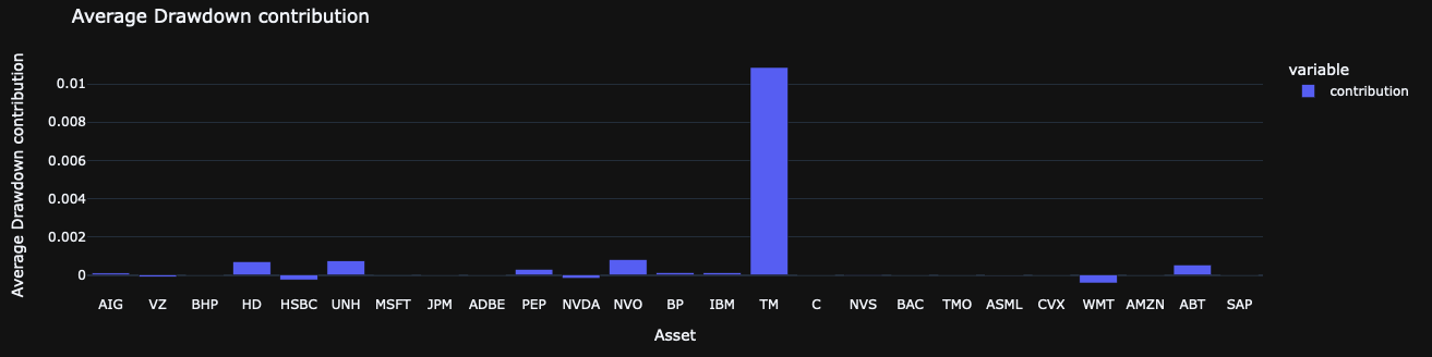
</code></pre>

<figure><img src="https://1304136543-files.gitbook.io/~/files/v0/b/gitbook-x-prod.appspot.com/o/spaces%2FCbqQ4ogM0YiEs5Z9Djdn%2Fuploads%2Fgit-blob-b1f6635b97d8dd129a573eebb4cff16d57b14385%2Fweight_optimization_9.png?alt=media" alt=""><figcaption></figcaption></figure>

### **Sharpe Ratio Contribution**

Indicates which assets contribute most to the portfolio's Sharpe ratio, highlighting return drivers.

<pre class="language-python"><code class="lang-python"><a data-footnote-ref href="#user-content-fn-1">portfolio</a>["model_name"].sharpe_contribution_plot
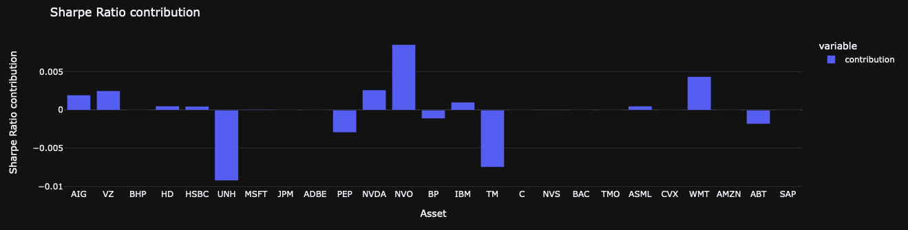
</code></pre>

<figure><img src="https://1304136543-files.gitbook.io/~/files/v0/b/gitbook-x-prod.appspot.com/o/spaces%2FCbqQ4ogM0YiEs5Z9Djdn%2Fuploads%2Fgit-blob-2664d30b95877388913448c6275c5b4625b53874%2Fweight_optimization_10.png?alt=media" alt=""><figcaption></figcaption></figure>

### **Correlation Heatmap**

Displays the correlation structure of assets used in the model (not available for EQUAL).

<pre class="language-python"><code class="lang-python"><a data-footnote-ref href="#user-content-fn-1">portfolio</a>["model_name"].heatmap_plot
</code></pre>

<figure><img src="https://1304136543-files.gitbook.io/~/files/v0/b/gitbook-x-prod.appspot.com/o/spaces%2FCbqQ4ogM0YiEs5Z9Djdn%2Fuploads%2Fgit-blob-c76679a358f904b2d3ec3e5c89fbb5c17bd5e471%2Fweight_optimization_11.png?alt=media" alt=""><figcaption></figcaption></figure>

### **Clustering Dendrogram**

Visualizes the hierarchical clustering of assets used in the model (not available for EQUAL).

<pre class="language-python"><code class="lang-python"><a data-footnote-ref href="#user-content-fn-1">portfolio</a>["model_name"].cluster_plot
</code></pre>

<figure><img src="https://1304136543-files.gitbook.io/~/files/v0/b/gitbook-x-prod.appspot.com/o/spaces%2FCbqQ4ogM0YiEs5Z9Djdn%2Fuploads%2Fgit-blob-163443fdafac99414a454ca46599261538e17309%2Fweight_optimization_12.png?alt=media" alt=""><figcaption></figcaption></figure>

### **Current Recommended Allocation**

Provides the model's most recent recommended asset allocation.

<pre class="language-python"><code class="lang-python"><a data-footnote-ref href="#user-content-fn-1">portfolio</a>["model_name"].recommended_allocation
</code></pre>

<figure><img src="https://1304136543-files.gitbook.io/~/files/v0/b/gitbook-x-prod.appspot.com/o/spaces%2FCbqQ4ogM0YiEs5Z9Djdn%2Fuploads%2Fgit-blob-91e7c82525ae144d9b18d6510b51f119f6e6dd89%2Fweight_optimization_13.png?alt=media" alt=""><figcaption></figcaption></figure>

### **Sharpe Ratio Distribution**

Shows the distribution of Sharpe ratio helping to understand the consistency of risk-adjusted returns.

<pre class="language-python"><code class="lang-python"><a data-footnote-ref href="#user-content-fn-1">portfolio</a>["model_name"].recommended_allocation
</code></pre>

<figure><img src="https://1304136543-files.gitbook.io/~/files/v0/b/gitbook-x-prod.appspot.com/o/spaces%2FCbqQ4ogM0YiEs5Z9Djdn%2Fuploads%2Fgit-blob-3cc6f9da7460ead176c682b46a1ffe4011a87300%2Fweight_optimization_14.png?alt=media" alt=""><figcaption></figcaption></figure>

### **Daily Weights**

Shows how the model's asset allocation changes day-by-day over the backtesting period.

<pre class="language-python"><code class="lang-python"><a data-footnote-ref href="#user-content-fn-1">portfolio</a>["model_name"].daily_weights
</code></pre>

<figure><img src="https://1304136543-files.gitbook.io/~/files/v0/b/gitbook-x-prod.appspot.com/o/spaces%2FCbqQ4ogM0YiEs5Z9Djdn%2Fuploads%2Fgit-blob-ac4e2b4f52732fc9ea56960d426e91df69f0f7f6%2Fweight_optimization_15.png?alt=media" alt=""><figcaption></figcaption></figure>

[^1]: class module


# Screens and Filters

This module allows users to apply various filters and screens to a comprehensive dataset of financial and market factors.

`Tutorials` are the best documentation — [<mark style="color:blue;">`Screens and Filters Tutorial`</mark>](https://colab.research.google.com/github/sovai-research/sovai-public/blob/main/notebooks/studies/Screens%20and%20Filters.ipynb)

## Screens and Filters Module

### Overview

The Screens and Filters module is a versatile component of the sovai software suite, designed to help investors and analysts identify novel investment opportunities using a wide range of features as filtering and selection criteria.

### Key Features

* Access to hundreds of financial and market factors
* Ability to filter based on latest data points
* Stock selection by market capitalization categories
* Flexible querying capabilities
* Chaining of multiple filters and selections

### Usage

To use the Screens and Filters module, you first need to authenticate and then you can start applying various filters and screens to the data. Here's an example of how to use this module:

```python
import sovai as sov

# Authenticate
sov.token_auth(token="your_authentication_token")

# Load comprehensive factor data
df_comprehensive = sov.data("factors/comprehensive")
```

### Available Methods and Functionality

#### 1. Get Latest Data

```python
df_risk = df_comprehensive.get_latest("business_risk")[["business_risk"]]
```

This method allows you to extract the most recent data point for a specific factor.

#### 2. Select Stocks by Market Cap

```python
df_mega = df_risk.select_stocks("mega")
```

This method filters stocks based on market capitalization category. In this example, it selects only mega-cap stocks.

#### 3. Apply Custom Queries

```python
df_ten = df_mega.query("business_risk <= 10")
```

This method allows you to apply custom filtering conditions using familiar Python query syntax.

#### 4. Chaining Operations

You can chain multiple operations together for more complex screening:

```python
df_ten = (sov.data("factors/comprehensive")
          .get_latest("business_risk")[["business_risk"]]
          .select_stocks("mega")
          .query("business_risk <= 10"))
```

This chain of operations:

1. Loads the comprehensive factor data
2. Selects the latest "business\_risk" factor
3. Filters for mega-cap stocks
4. Applies a custom query to select stocks with business risk <= 10

### Example Use Case

Let's walk through an example of using the Screens and Filters module to identify large-cap companies with low business risk sensitivity:

```python
import sovai as sov

# Authenticate
sov.token_auth(token="your_authentication_token")

# Load data, filter for mega-caps with business risk <= 10
df_filtered = (sov.data("factors/comprehensive")
               .get_latest("business_risk")[["business_risk"]]
               .select_stocks("mega")
               .query("business_risk <= 10"))

print(df_filtered)
```

This script will return a DataFrame containing mega-cap stocks with a business risk sensitivity of 10% or less, based on the most recent data point.

### Conclusion

The Screens and Filters module provides a powerful and flexible way to identify investment opportunities based on a wide range of factors. By combining different filtering methods and leveraging the extensive factor database, users can create sophisticated screening strategies to suit their investment criteria.


# Pairwise Distance

Pairwise statistics for distance and similarity between stocks in cross-section, time-series, and panel orientations.

`Tutorials` are the best documentation — [<mark style="color:blue;">`Pairwise Distance Tutorial`</mark>](https://colab.research.google.com/github/sovai-research/sovai-public/blob/main/notebooks/computational/Pairwise%20Distance.ipynb)

## Pairwise Distance Statistics Module

`dataframe.distance()`

### Tutorial for Context.

### Features

* Cross-sectional distance calculations
* Time-series distance calculations
* Panel data distance calculations (Tucker decomposition)
* Multiple distance metrics and statistical tests

### Usage

The module is integrated into a custom DataFrame class, allowing for easy calculation of pairwise distances.

```python
import sovai as sov

# Load data
df_factors = sov.data("factors/accounting")

# Select a subset of data
df_slice = df_factors.select_stocks("mega").date_range("2020-01-01")

# Calculate distances
dist_matrix = df_slice.distance()
```

<figure><img src="https://1304136543-files.gitbook.io/~/files/v0/b/gitbook-x-prod.appspot.com/o/spaces%2FCbqQ4ogM0YiEs5Z9Djdn%2Fuploads%2Fgit-blob-352b1f910c1bd72e2e4998bddeec0abf8a0a6e8b%2Fpairwise_distance_1.png?alt=media" alt=""><figcaption></figcaption></figure>

### Distance Calculation Methods

#### 1. Cross-Sectional Distance

Calculates distances between stocks based on their attributes at each time point.

```python
dist_matrix = df_slice.distance(orient="cross-sectional", distance='cosine', calculations=features)
```

**Parameters:**

* `orient`: Set to "cross-sectional"
* `distance`: Distance metric (e.g., 'cosine', 'euclidean')
* **`calculations`**: List of features to include in the distance calculation

**Available Calculations:**

* `mean`: Average value
* `skew`: Skewness
* `std`: Standard deviation
* `diffm`: First difference mean
* `zcr`: Zero crossing rate
* `mac`: Mean absolute change
* `sc`: Spectral centroid
* `tp`: Turning points
* `acl1`: Autocorrelation at lag 1
* `hjorthm`: Hjorth mobility
* `hurst`: Hurst exponent
* `hist`: Histogram mode (5 bins)
* `timerev`: Time reversibility statistic

#### 2. Time-Series Distance

Computes distances between stocks based on their time-series behavior.

```python
dist_matrix = df_slice.distance(orient="time-series", metric="pearson")
```

**Parameters:**

* `orient`: Set to "time-series"
* **`metric`**: Distance metric to use

**Available Metrics:**

* `pearson`: Pearson correlation
* `spearman`: Spearman correlation
* `dtw`: Dynamic Time Warping
* `euclidean`: Euclidean distance
* `euclidean_int`: Euclidean distance with interpolation
* `pec`: Power Envelope Correlation
* `frechet`: Fréchet distance
* `kl_divergence`: Kullback-Leibler divergence
* `wasserstein`: Wasserstein distance
* `jaccard`: Jaccard distance
* `bray_curtis`: Bray-Curtis dissimilarity
* `hausdorff`: Hausdorff distance
* `manhattan`: Manhattan distance
* `chi2`: Chi-squared distance
* `hellinger`: Hellinger distance
* `canberra`: Canberra distance
* `shannon_entropy`: Shannon entropy-based distance
* `sample_entropy`: Sample entropy
* `approx_entropy`: Approximate entropy
* `jensen_shannon`: Jensen-Shannon divergence
* `renyi_entropy`: Rényi entropy
* `tsallis_entropy`: Tsallis entropy
* `mutual_information`: Mutual information-based distance

#### 3. Panel Data Distance

Utilizes Tucker decomposition to calculate distances considering both cross-sectional and time-series aspects.

```python
dist_matrix = df_slice.distance(orient="panel")
```

**Parameters:**

* `orient`: Set to "panel"

### Notes

* The module handles missing values by imputing them with the median.
* Some distance calculations may be computationally intensive for large datasets.
* The Tucker decomposition for panel data provides an estimated rank of the decomposition.

### Example

```python
# Calculate cross-sectional distances
dist_matrix_all = df_slice.distance(orient="cross-sectional", distance='cosine', calculations=features)

# Calculate time-series distances using Pearson correlation
dist_matrix_pearson = df_slice.distance(orient="time-series", metric="pearson")

# Calculate panel data distances
dist_matrix_tucker = df_slice.distance(orient="panel")
```

### Date instead of Ticker

While previous examples focused on calculating distances between stocks, we can also compute distances between dates using the same methods.

This allows for analyzing how market conditions change over time.

### Converting to Date

All previous distance calculation functions can be modified to work with dates by specifying `on="date"`. Here are the key functions adapted for date-based analysis:

```python
# Mean distance between dates
dist_matrix_mean = df_slice.distance(on="date")

# Cross-sectional distances using cosine similarity
dist_matrix_cos = df_slice.distance(orient="cross-sectional", on="date", distance='cosine', calculations=features)

# Cross-sectional distances using Euclidean distance
dist_matrix_euc = df_slice.distance(orient="cross-sectional", on="date", distance='euclidean', calculations=features)

# Time-series distances using Pearson correlation
dist_matrix_pearson = df_slice.distance(orient="time-series", on="date", metric="pearson")

# Time-series distances using Dynamic Time Warping
dist_matrix_dtw = df_slice.distance(orient="time-series", on="date", metric="dtw")

# Time-series distances using Tsallis entropy
dist_matrix_tsent = df_slice.distance(orient="time-series", on="date", metric="tsallis_entropy")

# Panel data distances using Tucker decomposition
dist_matrix_tucker = df_slice.distance(orient="panel", on="date")
```

These functions calculate distances between different dates based on the market conditions or stock behaviors on those dates.

<figure><img src="https://1304136543-files.gitbook.io/~/files/v0/b/gitbook-x-prod.appspot.com/o/spaces%2FCbqQ4ogM0YiEs5Z9Djdn%2Fuploads%2Fgit-blob-0ea8b4ba7c614a9daa4e0d25fd620036ce74e571%2Fpairwise_distance_2.png?alt=media" alt=""><figcaption></figcaption></figure>

### Sorting and Analyzing Date Distances

To analyze the distances for a specific date:

```python
date = dist_matrix_cos.index.max()
dist_matrix_cos.sort_values(date)[[date]].T
```

This code:

1. Selects the most recent date
2. Sorts the distances for that date
3. Displays the results as a transposed row

The output shows how similar or different market conditions on other dates were compared to the selected date, allowing for temporal analysis of market behavior.

This approach can help identify patterns, trends, or anomalous periods in market history by comparing the similarity of market conditions across different dates


# Anomaly Detection

It provides methods to detect global, local, and cluster anomalies in multivariate financial data

`Tutorials` are the best documentation — [<mark style="color:blue;">`Anomaly Detection Tutorial`</mark>](https://colab.research.google.com/github/sovai-research/sovai-public/blob/main/notebooks/computational/Anomaly%20Detection.ipynb)

### Key Features

1. Multiple anomaly detection methods:
   * Global anomalies: Identify outliers considering the entire dataset
   * Local anomalies: Detect outliers within local neighborhoods
   * Cluster anomalies: Find anomalies considering multi-dimensional data structure
2. Anomaly scoring: Compute anomaly scores for each data point
3. Feature-level anomaly analysis: Identify the most anomalous features for a given security

### Usage

Load the accounting factors data:

```python
import pandas as pd

df_factors = sov.data("factors/accounting", purge_cache=True)
df_last_3_years = df_factors.loc[(slice(None), slice(pd.Timestamp.now() - pd.DateOffset(years=3), None)), :]
df_last_3_years = df_last_3_years.percentile()
```

### Anomaly Detection

#### Compute Anomaly Scores

<pre class="language-python"><code class="lang-python"><strong>df_anomaly_scores = df_last_3_years.anomalies("scores", ticker="TSLA")
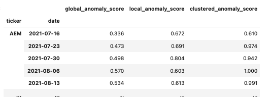
</strong></code></pre>

<figure><img src="https://1304136543-files.gitbook.io/~/files/v0/b/gitbook-x-prod.appspot.com/o/spaces%2FCbqQ4ogM0YiEs5Z9Djdn%2Fuploads%2Fgit-blob-e7076b9fc30593af271b7339fce52f83c3cd1c4f%2Fanomaly_detection_1.png?alt=media" alt=""><figcaption></figcaption></figure>

#### Local Anomalies

```python
df_local = df_last_3_years.anomalies("local", ticker="NVDA")
```

<figure><img src="https://1304136543-files.gitbook.io/~/files/v0/b/gitbook-x-prod.appspot.com/o/spaces%2FCbqQ4ogM0YiEs5Z9Djdn%2Fuploads%2Fgit-blob-f7e440162e2282aacb7cc23f01cf6d55ee385525%2Fanomaly_detection_2.png?alt=media" alt=""><figcaption></figcaption></figure>

#### Global Anomalies

```python
df_global = df_last_3_years.anomalies("global", ticker="NVDA")
```

<figure><img src="https://1304136543-files.gitbook.io/~/files/v0/b/gitbook-x-prod.appspot.com/o/spaces%2FCbqQ4ogM0YiEs5Z9Djdn%2Fuploads%2Fgit-blob-0c992fd4dd7c13145212ea3707a1828dafd54f5e%2Fanomaly_detection_3.png?alt=media" alt=""><figcaption></figcaption></figure>

#### Cluster Anomalies

```python
df_cluster = df_last_3_years.anomalies("cluster", ticker="NVDA")
```

<figure><img src="https://1304136543-files.gitbook.io/~/files/v0/b/gitbook-x-prod.appspot.com/o/spaces%2FCbqQ4ogM0YiEs5Z9Djdn%2Fuploads%2Fgit-blob-96c15f15a1b8c266fe29ae60fa18277da552b975%2Fanomaly_detection_4.png?alt=media" alt=""><figcaption></figcaption></figure>

### Notes

* The module uses the `sovai` library for data loading and processing. Ensure you have the necessary permissions and valid authentication token.
* Anomaly detection methods can be applied to different time ranges and tickers. Adjust the parameters as needed for your analysis.
* The module provides flexibility in analyzing anomalies at both the overall and feature level. Experiment with different combinations of methods for comprehensive insights.
* When working with large datasets, be mindful of computational resources, especially when applying multiple anomaly detection methods or creating complex visualizations.


# Clustering Panels

Clustering specifically designed for multivariate panel clustering of financial and time-series data

`Tutorials` are the best documentation — [<mark style="color:blue;">`Clustering Panels Tutorial`</mark>](https://colab.research.google.com/github/sovai-research/sovai-public/blob/main/notebooks/computational/Clustering%20Notebook.ipynb)

### Introduction

Can be used to cluster any panel dataset. It is particularly useful for financial analysts, data scientists, and researchers working with time-series data across multiple entities (e.g., stocks, companies) and variables.

#### Initialization

The CustomDataFrame can be initialized using the `sov.data()` function:

```python
import sovai as sov

sov.token_auth(token="your_token_here")
df = sov.data("accounting/weekly")
```

Basic Clustering

Perform clustering on all features:

```python
df_cluster = df.cluster()
```

<figure><img src="https://1304136543-files.gitbook.io/~/files/v0/b/gitbook-x-prod.appspot.com/o/spaces%2FCbqQ4ogM0YiEs5Z9Djdn%2Fuploads%2Fgit-blob-9f3998e1c3d51e31fc00c6b4386c84c2f5f59383%2Fclustering_panels_1.png?alt=media" alt=""><figcaption></figcaption></figure>

Feature-Specific Clustering

Cluster based on specific features:

```python
df_cluster_ebit = df.cluster(features=["ebit"])
df_cluster_multi = df.cluster(features=["total_assets", "total_debt", "ebit"])
```

#### Summary Clustering

Get a quick summary of the last 6-months data:

```python
df.cluster("summary")
```

<figure><img src="https://1304136543-files.gitbook.io/~/files/v0/b/gitbook-x-prod.appspot.com/o/spaces%2FCbqQ4ogM0YiEs5Z9Djdn%2Fuploads%2Fgit-blob-2e51671dd80d7a067905d5d93acdfebbd57eee9c%2Fclustering_panels_2.png?alt=media" alt=""><figcaption></figcaption></figure>

### Visualization Methods

#### Line Plot

Visualize cluster centroids and distances:

```python
df.cluster("line_plot")
```

<figure><img src="https://1304136543-files.gitbook.io/~/files/v0/b/gitbook-x-prod.appspot.com/o/spaces%2FCbqQ4ogM0YiEs5Z9Djdn%2Fuploads%2Fgit-blob-e3b1a6583e910d6cfdf7affd847fe8c4f3327fc9%2Fclustering_panels_3.png?alt=media" alt=""><figcaption></figcaption></figure>

**Scatter Plot**

Create a scatter plot of clustered data:

```python
df.cluster("scatter_plot")
```

<figure><img src="https://1304136543-files.gitbook.io/~/files/v0/b/gitbook-x-prod.appspot.com/o/spaces%2FCbqQ4ogM0YiEs5Z9Djdn%2Fuploads%2Fgit-blob-ec8603206a5e07319eadac2375a33adc979a7b8b%2Fclustering_panels_4.png?alt=media" alt=""><figcaption></figcaption></figure>

#### Animation Plot

Generate an animated plot of cluster evolution:

```python
df.cluster("animation_plot")
```

<figure><img src="https://1304136543-files.gitbook.io/~/files/v0/b/gitbook-x-prod.appspot.com/o/spaces%2FCbqQ4ogM0YiEs5Z9Djdn%2Fuploads%2Fgit-blob-0161e5a946c807ea4a0a817629285c133505f5bb%2Fclustering_panels_5.png?alt=media" alt=""><figcaption></figcaption></figure>

### Advanced Analysis

#### Distance Calculation

Calculate distances between ticker-cluster combinations:

```python
df_dist = df_cluster.drop(columns=["labels"]).distance(orient="time-series")
```

<figure><img src="https://1304136543-files.gitbook.io/~/files/v0/b/gitbook-x-prod.appspot.com/o/spaces%2FCbqQ4ogM0YiEs5Z9Djdn%2Fuploads%2Fgit-blob-83ecb2d84b60b2c647dca616a54e27773e0cfee1%2Fclustering_panels_6.png?alt=media" alt=""><figcaption></figcaption></figure>

### Examples

#### Basic Clustering and Visualization

```python
import sovai as sov

sov.token_auth(token="your_token_here")
df_accounting = sov.data("accounting/weekly")
df_mega = df_accounting.select_stocks("mega").date_range("2018-01-01")
df_cluster = df_mega.cluster()
df_mega.cluster("line_plot")
```

#### Feature-Specific Clustering and Distance Analysis

```python
df_cluster_ebit = df_mega.cluster(features=["ebit"])
df_dist = df_cluster_ebit.drop(columns=["labels"]).distance(orient="time-series")
similar_to_amzn = df_dist.sort_values(["AMZN"])[["AMZN"]].T
```


# Extract Features

The feature extractor module generates features that can be categorized into several types based on the nature of the calculations.

`Tutorials` are the best documentation — [<mark style="color:blue;">`Extract Features Tutorial`</mark>](https://colab.research.google.com/github/sovai-research/sovai-public/blob/main/notebooks/computational/Feature%20Extractions.ipynb)

## Feature Extraction Module

This module provides powerful feature extraction capabilities for time series data, particularly focused on financial and accounting metrics. It leverages the `sovai` library for data retrieval and a custom `feature_extractor` function for generating a wide range of statistical and time series features.

### Feature Categories

The `feature_extractor` generates features that fall into several categories:

* Statistical Features
* Entropy and Complexity Features
* Frequency and Streak Features
* Energy and Magnitude Features
* Distributional Features
* Position Features

### Usage Examples

```python
import sovai as sov

# Authenticate and load data
sov.token_auth(token="your_token_here")
df_mega = sov.data("accounting/weekly").select_stocks("mega").date_range("2018-01-01")
```

#### 1. Basic Usage with Default Parameters

```python
# Extract features with default parameters
result = df_mega.extract_features(every="all")
print(result.head())
```

<figure><img src="https://1304136543-files.gitbook.io/~/files/v0/b/gitbook-x-prod.appspot.com/o/spaces%2FCbqQ4ogM0YiEs5Z9Djdn%2Fuploads%2Fgit-blob-07f931e98b17efe1084f3ae721b9086ecae3663d%2Fextract_features_1.png?alt=media" alt=""><figcaption></figcaption></figure>

#### 2. Weekly Rolling Features

```python
# Extract features with a 12-week lookback, calculated weekly
result = df_mega.extract_features(lookback=12, every='week')
print(result.head())
```

#### 3. Custom Feature List

```python
# Extract specific features with custom parameters
custom_features = ["operating_working_capital", "cash_short_term"]
result = df_mega.extract_features(lookback=12, every='week', features=custom_features)
print(result.head())
```

#### 4. Monthly Rolling Features

```python
# Use monthly rolling features with a 2-month lookback
result = df_mega.extract_features(lookback='2mo', every='month')
print(result.head())
```

### Advanced Usage

The underlying `feature_extractor` function offers more granular control over the feature extraction process. It can be used directly for more advanced use cases:

```python
import polars as pl
from feature_extractor import feature_extractor

# Assuming df is your input DataFrame
result = feature_extractor(df, entity_col='ticker', date_col='date', 
                           lookback='1mo', every='week', verbose=True)
print(result.head())
```

This advanced usage allows for more customization, including specifying entity and date columns, adjusting lookback periods, and enabling verbose output for debugging.

#### Statistical Features

* **Mean and Variance Related:**
  * `mean_abs_change`
  * `variation_coefficient`
  * `mean_change`
  * `mean_second_derivative_central`

#### Entropy and Complexity Features

* **Entropy:**
  * `binned_entropy`
* **Complexity:**
  * `lempel_ziv_complexity`

#### Frequency and Streak Features

* **Frequency:**
  * `number_crossings`
  * `number_peaks`
* **Streak:**
  * `longest_streak_above_mean`
  * `longest_losing_streak`
  * `longest_winning_streak`

#### Energy and Magnitude Features

* **Energy:**
  * `absolute_energy`
* **Magnitude:**
  * `absolute_maximum`
  * `absolute_sum_of_changes`
  * `max_abs_change`

#### Statistical and Distributional Features

* **Statistical:**
  * `root_mean_square`
  * `ratio_beyond_r_sigma`
* **Distributional:**
  * `benford_correlation`
  * `percent_reoccurring_points`
  * `percent_reoccurring_values`

#### Position Features

* **Positions:**
  * `first_location_of_maximum`
  * `first_location_of_minimum`
  * `last_location_of_maximum`
  * `last_location_of_minimum`

These categories help organize the wide range of features generated, which capture different aspects of the time series data, making them useful for various analytical and predictive tasks.


# Neutralize Features

The feature extractor module generates features that can be categorized into several types based on the nature of the calculations.

`Tutorials` are the best documentation — [<mark style="color:blue;">`Neutralize Features Tutorial`</mark>](https://colab.research.google.com/github/sovai-research/sovai-public/blob/main/notebooks/computational/Feature%20Neutralization.ipynb)

## Feature Neutralization[¶](http://localhost:8888/lab/tree/notebooks/computational/Feature%20Neutralization.ipynb#Feature-Neutralization) <a href="#feature-neutralization" id="feature-neutralization"></a>

All these methods return the same number of columns as the input DataFrame. They transform the data while maintaining the original dimensionality, which is crucial for many financial applications where each feature represents a specific economic or financial metric.

1. Orthogonalization might be preferred when you want to remove correlations but keep the overall structure of the data. `orthogonalize_features`
2. Neutralization might be used when you want to focus on the unique aspects of each feature, removing common market factors. `neutralize_features`

#### Data Loading and Preparation

First, we load the necessary library and authenticate. Then we load the accounting data for mega-cap stocks from 2018 onwards.

```python
import sovai as sov

sov.token_auth(token="your_token_here")

# Load weekly accounting data
df_accounting = sov.data("accounting/weekly")

# Select mega-cap stocks from 2018 onwards
df_mega = df_accounting.select_stocks("mega").date_range("2018-01-01")
```

#### Orthogonalization

Orthogonalization transforms a set of features into a new set of uncorrelated (perpendicular) features while preserving the original information content. We demonstrate two methods: Gram-Schmidt and QR decomposition.

1. Gram-Schmidt method:

```python
# Apply Gram-Schmidt orthogonalization
df_orthogonalized_gs = df_mega.orthogonalize_features(method='gram_schmidt')
```

<figure><img src="https://1304136543-files.gitbook.io/~/files/v0/b/gitbook-x-prod.appspot.com/o/spaces%2FCbqQ4ogM0YiEs5Z9Djdn%2Fuploads%2Fgit-blob-9e8132c216f7ce7202c15e5161e53ab2fa3b4531%2Fneutralize_features_1.png?alt=media" alt=""><figcaption></figcaption></figure>

2. QR method:

```python
# Apply QR orthogonalization
df_orthogonalized_qr = df_mega.orthogonalize_features(method='qr')
```

#### Neutralization

Neutralization reduces the influence of common factors across features, typically by removing one or more principal components, leaving only the unique aspects of each feature. We demonstrate three methods: PCA, SVD, and Iterative Regression.

1. PCA method:

```python
# Apply PCA neutralization
df_neutralized_pca = df_mega.neutralize_features(method='pca')
```

2. SVD method:

```python
# Apply SVD neutralization
df_neutralized_svd = df_mega.neutralize_features(method='svd')
```

### Orthogonalization Methods:

* Gram-Schmidt orthogonalization:
  * Transforms the original features into a set of orthogonal features.
  * Each new feature is uncorrelated with all previous features.
  * Preserves the original information content but in a different coordinate system.
* QR decomposition:
  * Similar to Gram-Schmidt, it produces orthogonal features.
  * It's a more numerically stable method for orthogonalization.

### Neutralization Methods:

* PCA neutralization:
  * Transforms the data into principal components and keeps only the last component.
  * This effectively removes the main sources of variation in the data.
* SVD (Singular Value Decomposition) neutralization:
  * Similar to PCA, but uses SVD to decompose the data.
  * Keeps only the component associated with the smallest singular value.


# Select Features

The feature selection module in the sovai library provides various methods to identify and select the most important features from financial datasets.

`Tutorials` are the best documentation — [<mark style="color:blue;">`Select Features Tutorial`</mark>](https://colab.research.google.com/github/sovai-research/sovai-public/blob/main/notebooks/computational/Feature%20Selection.ipynb)

### Feature Selection Methods

The module supports several methods for feature selection, each based on different algorithms for determining feature importance. All methods use the `select_features` function with the following syntax:

```python
df_mega.select_features(method, n_components=10)
```

Where `method` is one of the following:

#### 1. Random Projection

```python
df_mega.select_features("random_projection", n_components=10)
```

Selects features based on their contribution to variance in the randomly projected space.

#### 2. Random Fourier Features

```python
df_mega.select_features("fourier", n_components=10)
```

Chooses features based on their influence on non-linear relationships in the Fourier-transformed space.

#### 3. Independent Component Analysis (ICA)

```python
df_mega.select_features("ica", n_components=10)
```

Selects features based on their contribution to extracted independent components, representing underlying independent signals in the data.

#### Truncated Singular Value Decomposition (SVD)

```python
df_mega.select_features("svd", n_components=10)
```

Chooses features based on their influence on principal singular vectors, which represent directions of maximum variance in the data.

#### Sparse Random Projection

```python
df_mega.select_features("sparse_projection", n_components=10)
```

Selects features based on their contribution to variance in the sparsely projected space, offering improved computational efficiency over standard Random Projection.

#### Clustered SHAP Ensemble

```python
df_mega.select_features("shapley", n_components=10)
```

Selects features using a method that iteratively applies clustering, uses XGBoost to predict cluster membership, calculates SHAP values, and averages results across multiple runs.

### Variability-based Selection

For all the models you can also select the number of components based on the total importance explained. When `variability` is specified:

```python
df_mega.select_features("random_projection", variability=0.80)
```

### Parameters

* `method`: String specifying the feature selection method (options listed above).
* `n_components`: Integer specifying the number of features to select (default is 10).
* If `variability` is provided, it must be a float between 0 and 1.

### Return Value

Each method returns a DataFrame containing the selected features and their corresponding data.

### Usage Notes

1. The `n_components` parameter allows you to control the number of features selected. Adjust this based on your specific needs and the total number of features in your dataset.
2. Different methods may yield different sets of selected features. It's often beneficial to compare results from multiple methods to gain a comprehensive understanding of feature importance.
3. The computational time may vary between methods. Some methods (like Sparse Random Projection) are designed for improved efficiency and may be preferable for larger datasets.
4. Always ensure you have sufficient historical data for reliable feature selection, especially when using methods that rely on capturing underlying data structures or relationships.
5. The selected features represent those deemed most important by each method. However, domain knowledge should also be considered when making final feature selection decisions for your specific application.


# Dimensionality Reduction

Implements multiple reduction techniques including PCA, SVD, Factor Analysis, Gaussian Random Projection, and UMAP.

`Tutorials` are the best documentation — [<mark style="color:blue;">`Dimensionality Reduction Tutorial`</mark>](https://colab.research.google.com/github/sovai-research/sovai-public/blob/main/notebooks/computational/Dimensionality%20Reduction.ipynb)

### Reduction Techniques

The module supports the following dimensionality reduction methods:

* PCA (Principal Component Analysis)
* Factor Analysis
* Gaussian Random Projection
* UMAP (Uniform Manifold Approximation and Projection)

### Usage Examples.

#### Authenticate and load data

```python
import sovai as sov
sov.token_auth(token="your_token_here")
df_mega = sov.data("accounting/weekly").select_stocks("mega").date_range("2018-01-01") 
```

#### 1. Basic Usage with PCA

```python
# Reduce dimensions using PCA
result = df_mega.reduce_dimensions(method="pca", n_components=10)
print(result.head())
```

#### 2. Using Gaussian Random Projection

```python
# Reduce dimensions using Gaussian Random Projection
result = df_mega.reduce_dimensions(method="gaussian_random_projection", n_components=10)
print(result.head())
```

#### 3. UMAP with Verbose Output

```python
# Reduce dimensions using UMAP with verbose output
result = df_mega.reduce_dimensions(method="umap", verbose=True, n_components=10)
print(result.head())
```

#### 4. Factor Analysis

```python
# Reduce dimensions using Factor Analysis with verbose output
result = df_mega.reduce_dimensions(method="factor_analysis", verbose=True, n_components=10)
print(result.head())
```

### Advanced Usage

The underlying `dimensionality_reduction` function offers more control over the reduction process:

```python
from dimensionality_reduction import dimensionality_reduction

# Assuming df is your input DataFrame
result = dimensionality_reduction(df, method='pca', explained_variance=0.95, verbose=True)
print(result.head())
```

This advanced usage allows for specifying the amount of variance to be explained if `n_components` is not provided.

### Performance Considerations

* The dimensionality reduction process can be computationally intensive, especially for large datasets or when using methods like UMAP.
* PCA and Truncated SVD are generally faster than UMAP for large datasets.
* Consider using a smaller number of components or a subset of your data if performance is a concern.


# Feature Importance

The feature importance module in the sovai library offers multiple unsupervised algorithms to quantify the significance of each feature in financial datasets.

`Tutorials` are the best documentation — [<mark style="color:blue;">`Feature Importance Tutorial`</mark>](https://colab.research.google.com/github/sovai-research/sovai-public/blob/main/notebooks/computational/Feature%20Importance.ipynb)

### Feature Importance Methods

The module supports several methods for calculating feature importance:

#### Random Projection

```python
df_mega.importance("random_projection")
```

<figure><img src="https://1304136543-files.gitbook.io/~/files/v0/b/gitbook-x-prod.appspot.com/o/spaces%2FCbqQ4ogM0YiEs5Z9Djdn%2Fuploads%2Fgit-blob-8472b930bb23216d06c5bd7f509d9cf917a20002%2Ffeature_importance_1.png?alt=media" alt=""><figcaption></figcaption></figure>

Reflects how much each feature contributes to the variance in the randomly projected space.

#### Random Fourier Features

```python
df_mega.importance("fourier")
```

Indicates how strongly each feature influences the approximation of non-linear relationships in the Fourier-transformed space.

#### Independent Component Analysis (ICA)

```python
df_mega.importance("ica")
```

Based on the magnitude of each feature's contribution to the extracted independent components, representing underlying independent signals in the data.

#### Truncated Singular Value Decomposition (SVD)

```python
df_mega.importance("svd")
```

Determined by each feature's influence on the principal singular vectors, which represent directions of maximum variance in the data.

#### Sparse Random Projection

```python
df_mega.importance("sparse_projection")
```

Based on how much each feature contributes to the variance in the sparsely projected space, similar to standard Random Projection but with improved computational efficiency.

#### Clustered SHAP Ensemble

```python
df_mega.importance("shapley")
```

Iteratively applies clustering, uses XGBoost to predict cluster membership, calculates SHAP values, and averages results across multiple runs to determine feature importance in identifying natural data structures.

### Global Feature Importance

To calculate global feature importance across all methods:

```python
df_mega.feature_importance()
```

### Feature Selection

Example of selecting top features based on importance scores:

```python
feature_importance = df_mega.importance("sparse_projection")
df_select = df_mega[feature_importance["feature"].head(25)]
```

<figure><img src="https://1304136543-files.gitbook.io/~/files/v0/b/gitbook-x-prod.appspot.com/o/spaces%2FCbqQ4ogM0YiEs5Z9Djdn%2Fuploads%2Fgit-blob-9437f5b64612c2d3bbd398eb057582006b363763%2Ffeature_importance_2.png?alt=media" alt=""><figcaption></figcaption></figure>


# Nowcasting Series

This module provides functionality for nowcasting financial data using a Multi-Frequency Long-term and Event-based forecasting method.

`Tutorials` are the best documentation — [<mark style="color:blue;">`Nowcasting Series Tutorial`</mark>](https://colab.research.google.com/github/sovai-research/sovai-public/blob/main/notebooks/computational/Nowcasting%20Notebook.ipynb)

## Nowcasting Module

This module demonstrates how to use the `sovai` library for nowcasting financial data, particularly focusing on accounting data for mega-cap stocks.

### Setup

First, import and authenticate with the `sovai` library:

### Nowcasting

#### For a Specific Stock

To perform nowcasting for a particular stock (e.g., AAPL) and a specific accounting metric (e.g., accounts receivable):

```python
df_accounting.query("ticker == 'AAPL'").nowcast("data", "accounts_receivable")
```

#### For All Stocks

To perform nowcasting for all stocks in the dataset:

```python
df_accounting.nowcast("data", "accounts_receivable")
```

### Visualization

To create a plot of the nowcasted data:

```python
df_accounting.nowcast("plot")
```

<figure><img src="https://1304136543-files.gitbook.io/~/files/v0/b/gitbook-x-prod.appspot.com/o/spaces%2FCbqQ4ogM0YiEs5Z9Djdn%2Fuploads%2Fgit-blob-442cbec3605a46e1de3b05971d80cf28d44cb454%2Fnowcasting_series_1.png?alt=media" alt=""><figcaption></figcaption></figure>

### Notes

* The `sovai` library provides methods for data retrieval, stock selection, and nowcasting.
* The `nowcast` method can be used with "data" parameter to return nowcasted data, or "plot" to generate a visualization.
* Make sure you have the necessary permissions and a valid token to access the `sovai` library and its data.

This notebook demonstrates a streamlined approach to nowcasting financial data using the `sovai` library, allowing for quick analysis of accounting metrics for mega-cap stocks.


# TS Decomposition

This module provides powerful tools for analyzing financial time series data, offering insights that can be valuable for financial analysis, investment decision-making, and economic research.

`Tutorials` are the best documentation — [<mark style="color:blue;">`Time Series Decomposition Tutorial`</mark>](https://colab.research.google.com/github/sovai-research/sovai-public/blob/main/notebooks/computational/Decomposition%20Notebook.ipynb)

### Decomposition Techniques

The module primarily uses the Multiple Seasonal-Trend decomposition using LOESS method, which allows for:

* Trend extraction
* Multiple seasonal component extraction (e.g., weekly, monthly, quarterly)
* Remainder (residual) calculation

### Reactive Trend Analysis

This feature categorizes the trend in real-time as:

* Increasing
* Decreasing
* Sideways

### Usage Examples

```python
import sovai as sov

# Authenticate and load data
sov.token_auth(token="your_token_here")

df_accounting = sov.data("accounting/weekly").select_stocks("mega")
```

### Time Decomposition and Statistrics

<figure><img src="https://1304136543-files.gitbook.io/~/files/v0/b/gitbook-x-prod.appspot.com/o/spaces%2FCbqQ4ogM0YiEs5Z9Djdn%2Fuploads%2Fgit-blob-41b0d4c6eb8cf5e0da6f236e1e3fd9f0ec086657%2Finstitutional_1_1.png?alt=media" alt=""><figcaption></figcaption></figure>

```python
# Perform time decomposition
df_time = df_accounting.time_decomposition(method="data", ticker="AAPL", feature="total_revenue")
# Access overall statistics
```

```
print(df_time.attrs["stats"])
```

####

### Interactive Dashboard

```python
# Generate decomposition plot
df_accounting.time_decomposition(method="plot", ticker="AAPL", feature="total_revenue")
```

<figure><img src="https://1304136543-files.gitbook.io/~/files/v0/b/gitbook-x-prod.appspot.com/o/spaces%2FCbqQ4ogM0YiEs5Z9Djdn%2Fuploads%2Fgit-blob-2e94713bf06c062d14e61cc37948ebb11b200878%2Finstitutional_1_2.png?alt=media" alt=""><figcaption></figcaption></figure>


# Time Segmentation

Segments time series into different components according to statistical tests over the series. Helpful for understanding changes in regimes.

`Tutorials` are the best documentation — [<mark style="color:blue;">`Time Segmentation Tutorial`</mark>](https://colab.research.google.com/github/sovai-research/sovai-public/blob/main/notebooks/computational/Segmentation%20Notebook.ipynb)

### Overview

The Time Segmentation Module is a powerful tool for analyzing financial time series data. It offers four main functionalities:

1. Change Point Detection
2. Regime Change Analysis
3. Comprehensive Regime Analysis (PCA-based)

Each functionality can be used for data analysis or visualization, allowing users to gain deep insights into their financial data.

### Getting Started

To use the Time Segmentation Module, first import the necessary library and authenticate:

```python
import sovai as sov
sov.token_auth(token="your_token_here")
```

```python
df_accounting = sov.data("accounting/weekly").select_stocks("mega")
```

### 1. Change Point Detection

Identify significant changes in your time series data.

#### Data Analysis

```python
df_change = df_accounting.change_point(method='data', feature="book_equity_value")
df_change.tail(10)  # View the last 10 rows
df_change.attrs['stats']  # View additional statistics
```

<figure><img src="https://1304136543-files.gitbook.io/~/files/v0/b/gitbook-x-prod.appspot.com/o/spaces%2FCbqQ4ogM0YiEs5Z9Djdn%2Fuploads%2Fgit-blob-d753017ea30b3fdf4f1ab5c54fe807d1bb999c5a%2Ftime_segmentation_1.png?alt=media" alt=""><figcaption></figcaption></figure>

#### Visualization

```python
df_accounting.change_point(method='plot')
```

<figure><img src="https://1304136543-files.gitbook.io/~/files/v0/b/gitbook-x-prod.appspot.com/o/spaces%2FCbqQ4ogM0YiEs5Z9Djdn%2Fuploads%2Fgit-blob-7490914898f38adde88dea7d1b7a297158eb733b%2Ftime_segmentation_2.png?alt=media" alt=""><figcaption></figcaption></figure>

### 2. Regime Change Analysis

Detect regime changes for a specific stock and feature.

#### Data Analysis

```python
rc_result = df_accounting.regime_change(method="data", ticker="AAPL", feature="total_revenue")
rc_result.tail(10)  # View the last 10 rows
rc_result.attrs['stats']  # View additional statistics
```

<figure><img src="https://1304136543-files.gitbook.io/~/files/v0/b/gitbook-x-prod.appspot.com/o/spaces%2FCbqQ4ogM0YiEs5Z9Djdn%2Fuploads%2Fgit-blob-a071fbb9f879207764b5dc037fe05f5b0f4a5c45%2Ftime_segmentation_3.png?alt=media" alt=""><figcaption></figcaption></figure>

#### Visualization

```python
df_accounting.regime_change(method="plot", ticker="AAPL", feature="total_revenue")
```

<figure><img src="https://1304136543-files.gitbook.io/~/files/v0/b/gitbook-x-prod.appspot.com/o/spaces%2FCbqQ4ogM0YiEs5Z9Djdn%2Fuploads%2Fgit-blob-25d37e83e420f6e128a943e91ba0dd291d8d1801%2Ftime_segmentation_4.png?alt=media" alt=""><figcaption></figcaption></figure>

### 3. Comprehensive Regime Analysis (PCA-based)

Perform a PCA-based regime change analysis on multiple features for a specific stock.

#### Data Analysis

```python
pca_rc_result = df_accounting.pca_regime_change(method="data", ticker="AAPL")
pca_rc_result.tail()  # View the last rows
pca_rc_result.attrs['stats']  # View additional statistics
```

<figure><img src="https://1304136543-files.gitbook.io/~/files/v0/b/gitbook-x-prod.appspot.com/o/spaces%2FCbqQ4ogM0YiEs5Z9Djdn%2Fuploads%2Fgit-blob-629aa388d7ba19e05f8388934318ce2aa45ac429%2Ftime_segmentation_5.png?alt=media" alt=""><figcaption></figcaption></figure>

#### Visualization

```python
df_accounting.pca_regime_change(method="plot", ticker="AAPL")
```

<figure><img src="https://1304136543-files.gitbook.io/~/files/v0/b/gitbook-x-prod.appspot.com/o/spaces%2FCbqQ4ogM0YiEs5Z9Djdn%2Fuploads%2Fgit-blob-a8fd99ccbffc9471fc099ecb0b3d02db766c4874%2Ftime_segmentation_6.png?alt=media" alt=""><figcaption></figcaption></figure>

### Tips for Users

* Always check the `.attrs['stats']` of the result for additional insights and metadata.
* Use the 'plot' method for quick visual analysis and the 'data' method for detailed numerical results.
* Experiment with different features and tickers to gain comprehensive insights into your financial data.

***


# Bankruptcy Prediction

Example of the type of dashboard that can be built using the underlying bankruptcy data. Get in touch to develop your own dashboard.

### [Bankruptcy Predictions](https://sov.ai/app/get/bankruptcies/predictions)

<figure><img src="https://1304136543-files.gitbook.io/~/files/v0/b/gitbook-x-prod.appspot.com/o/spaces%2FCbqQ4ogM0YiEs5Z9Djdn%2Fuploads%2Fgit-blob-ee4f6e78650a61201fd669275649a30582ee9a29%2Fbankruptcy_prediction_1.png?alt=media" alt=""><figcaption></figcaption></figure>

### [Bankruptcy Explanations](https://sov.ai/app/get/bankruptcies/explanation)

<figure><img src="https://1304136543-files.gitbook.io/~/files/v0/b/gitbook-x-prod.appspot.com/o/spaces%2FCbqQ4ogM0YiEs5Z9Djdn%2Fuploads%2Fgit-blob-e9ad5bc4c120887961eb1a273234c170938956ae%2Fbankruptcy_prediction_2.png?alt=media" alt=""><figcaption></figcaption></figure>

### [Model Performance](https://sov.ai/app/get/bankruptcies/performance)

<figure><img src="https://1304136543-files.gitbook.io/~/files/v0/b/gitbook-x-prod.appspot.com/o/spaces%2FCbqQ4ogM0YiEs5Z9Djdn%2Fuploads%2Fgit-blob-34b1e4752a800d4e4fa2998866aee62c601e8a48%2Fbankruptcy_prediction_3.png?alt=media" alt=""><figcaption></figcaption></figure>


# Turing Risk Index

Example of the type of dashboard that can be built using the underlying turing risk data. Get in touch to develop your own dashboard.

### [Overall Index](https://sov.ai/app/get/overall-index)

<figure><img src="https://1304136543-files.gitbook.io/~/files/v0/b/gitbook-x-prod.appspot.com/o/spaces%2FCbqQ4ogM0YiEs5Z9Djdn%2Fuploads%2Fgit-blob-3e7abee645477812f754bd51dedbdb1efaa96ddb%2Fturing_risk_index_1.png?alt=media" alt=""><figcaption></figcaption></figure>

### [Index Composition](https://sov.ai/app/get/index-composition)

<figure><img src="https://1304136543-files.gitbook.io/~/files/v0/b/gitbook-x-prod.appspot.com/o/spaces%2FCbqQ4ogM0YiEs5Z9Djdn%2Fuploads%2Fgit-blob-301fff94c5f2507064c6824d969cddac059ffdbe%2Fturing_risk_index_2.png?alt=media" alt=""><figcaption></figcaption></figure>

### [Risk Forecast](https://sov.ai/app/get/risk-forecast)

<figure><img src="https://1304136543-files.gitbook.io/~/files/v0/b/gitbook-x-prod.appspot.com/o/spaces%2FCbqQ4ogM0YiEs5Z9Djdn%2Fuploads%2Fgit-blob-da8b6614aa6441830b06921b191e26d996575d2d%2Fturing_risk_index_3.png?alt=media" alt=""><figcaption></figcaption></figure>

### [Risk Statistics](https://sov.ai/app/get/risk-statistics)

<figure><img src="https://1304136543-files.gitbook.io/~/files/v0/b/gitbook-x-prod.appspot.com/o/spaces%2FCbqQ4ogM0YiEs5Z9Djdn%2Fuploads%2Fgit-blob-c800648f41b295a8603a9033d0968b406a98e31f%2Fturing_risk_index_4.png?alt=media" alt=""><figcaption></figcaption></figure>


# API Overview

Complete API reference for the SovAI Python SDK, auto-generated from source code.

This section contains auto-generated API documentation for the `sovai` Python SDK.

Every public function, class, and module is documented with its signature, parameters, return types, and docstring.

## Core API

| Function                                  | Description                             |
| ----------------------------------------- | --------------------------------------- |
| [`sov.data()`](/api-reference/data)       | Retrieve data from 50+ endpoints        |
| [`sov.plot()`](/api-reference/plots)      | Generate pre-built visualizations       |
| [`sov.report()`](/api-reference/reports)  | Generate analytical reports             |
| [`sov.compute()`](/api-reference/compute) | Run computations on data                |
| [`sov.explain()`](/api-reference/tools)   | AI-powered chart and table explanations |

## Authentication

| Function                                        | Description                      |
| ----------------------------------------------- | -------------------------------- |
| [`sov.token_auth()`](/api-reference/token-auth) | Authenticate with API token      |
| [`sov.basic_auth()`](/api-reference/basic-auth) | Authenticate with email/password |
| [`sov.read_key()`](/api-reference/api-config)   | Read token from .env file        |

## Extensions

The [Extensions](/api-reference/extensions) module adds analytics methods directly to DataFrames: anomaly detection, clustering, feature extraction, signal evaluation, and more.

## Plot Library

The [Plot Library](/api-reference/plots-1) contains 50+ pre-built chart types organized by dataset category.


# sovai (Package)

Main SovAI SDK Tool Kit package

**Module:** `sovai`

Main SovAI SDK Tool Kit package

## Functions

### `data()`

```python
def data(args = (), kwargs = {})
```

Lazy-loaded access to the data function.

**Parameters**

| Parameter | Type | Description   |
| --------- | ---- | ------------- |
| `args`    | —    | Default: `()` |
| `kwargs`  | —    | Default: `{}` |

***


# Data Retrieval

API reference for sovai.get\_data

**Module:** `sovai.get_data`

## Classes

### `ApiRequestHandler`

```python
class ApiRequestHandler
```

Centralized handler for API requests with robust error handling, automatic retry capability, and consistent response processing.

This class encapsulates all HTTP communication logic, providing:

* Consistent authentication and headers
* Configurable retry policies with exponential backoff
* Proper error handling and logging
* Timeout management

**Attributes**

* `base_url`
* `token`
* `verify_ssl`
* `max_retries`
* `backoff_factor`
* `timeout`
* `headers` (`Dict[str, str]`)
* `logger`

**Methods**

### `__init__()`

```python
def __init__(
    self,
    base_url: str,
    token: str,
    verify_ssl: bool = True,
    max_retries: int = 3,
    backoff_factor: float = 0.5,
    timeout: tuple = (5, 30),
    logger: Optional[logging.Logger] = None,
)
```

Initialize the API request handler.

**Parameters**

| Parameter  | Type  | Description                                                                                                                                                                                                                                                                                                                                                             |
| ---------- | ----- | ----------------------------------------------------------------------------------------------------------------------------------------------------------------------------------------------------------------------------------------------------------------------------------------------------------------------------------------------------------------------- |
| `base_url` | `str` | Base URL for the API token: Authentication token verify\_ssl: Whether to verify SSL certificates max\_retries: Maximum number of retry attempts for failed requests backoff\_factor: Factor to determine wait time between retries timeout: Tuple of (connection timeout, read timeout) in seconds logger: Optional logger instance; uses module logger if not provided |

***

### `get()`

```python
def get(
    self,
    endpoint: str,
    params: Optional[Dict[str, Any]] = None,
    stream: bool = False,
    body: Optional[Dict[str, Any]] = None,
) -> requests.Response
```

Make a GET request to the API with proper error handling and retry logic.

**Parameters**

| Parameter  | Type  | Description                                                                                                   |
| ---------- | ----- | ------------------------------------------------------------------------------------------------------------- |
| `endpoint` | `str` | API endpoint path params: Query parameters stream: Whether to stream the response body: Optional request body |

**Returns**

requests.Response object

***

***

## Functions

### `data()`

```python
def data(
    endpoint: str,
    tickers: Optional[Union[str, List[str]]] = None,
    chart: Optional[str] = None,
    columns: Optional[Union[str, List[str]]] = None,
    version: Optional[str] = None,
    start_date: Optional[str] = None,
    end_date: Optional[str] = None,
    plot: bool = False,
    limit: Optional[int] = None,
    params: Optional[Dict[str, Any]] = None,
    body: Optional[Dict[str, Any]] = None,
    use_polars: bool = False,
    purge_cache: bool = False,
    parquet: bool = True,
    frequency: Optional[str] = None,
    verbose: bool = False,
    full_history: bool = False,
    source: Optional[str] = None,
) -> Union[DataFrameType, go.Figure, None]
```

Main function to retrieve data from the API. Caches results to disk in 'cache/' directory (Parquet for DataFrames, Pickle for Figures). Cache files older than 12 hours are automatically cleaned up.

**Parameters**

| Parameter      | Type                              | Description      |
| -------------- | --------------------------------- | ---------------- |
| `endpoint`     | `str`                             | —                |
| `tickers`      | `Optional[Union[str, List[str]]]` | Default: `None`  |
| `chart`        | `Optional[str]`                   | Default: `None`  |
| `columns`      | `Optional[Union[str, List[str]]]` | Default: `None`  |
| `version`      | `Optional[str]`                   | Default: `None`  |
| `start_date`   | `Optional[str]`                   | Default: `None`  |
| `end_date`     | `Optional[str]`                   | Default: `None`  |
| `plot`         | `bool`                            | Default: `False` |
| `limit`        | `Optional[int]`                   | Default: `None`  |
| `params`       | `Optional[Dict[str, Any]]`        | Default: `None`  |
| `body`         | `Optional[Dict[str, Any]]`        | Default: `None`  |
| `use_polars`   | `bool`                            | Default: `False` |
| `purge_cache`  | `bool`                            | Default: `False` |
| `parquet`      | `bool`                            | Default: `True`  |
| `frequency`    | `Optional[str]`                   | Default: `None`  |
| `verbose`      | `bool`                            | Default: `False` |
| `full_history` | `bool`                            | Default: `False` |
| `source`       | `Optional[str]`                   | Default: `None`  |

**Returns:** `Union[DataFrameType, go.Figure, None]`

***


# Plotting

API reference for sovai.get\_plots

**Module:** `sovai.get_plots`

## Functions

### `plot()`

```python
def plot(
    dataset_name,
    chart_type = None,
    df = None,
    tickers: Optional[List[str]] = None,
    ticker: Optional[str] = None,
    verbose = False,
    purge_cache = False,
    kwargs = {},
)
```

Generates plots based on dataset name and chart type. Lazily loads required plotting modules.

**Parameters**

| Parameter      | Type                  | Description      |
| -------------- | --------------------- | ---------------- |
| `dataset_name` | —                     | —                |
| `chart_type`   | —                     | Default: `None`  |
| `df`           | —                     | Default: `None`  |
| `tickers`      | `Optional[List[str]]` | Default: `None`  |
| `ticker`       | `Optional[str]`       | Default: `None`  |
| `verbose`      | —                     | Default: `False` |
| `purge_cache`  | —                     | Default: `False` |
| `kwargs`       | —                     | Default: `{}`    |

***


# Reports

API reference for sovai.get\_reports

**Module:** `sovai.get_reports`

## Functions

### `report()`

```python
def report(dataset_name, report_type = 'sector-top', kwargs = {})
```

***


# Compute

API reference for sovai.get\_compute

**Module:** `sovai.get_compute`

## Functions

### `compute()`

```python
def compute(compute_name = None, df = None, kwargs = {})
```

***


# Tools (SEC, Explain)

API reference for sovai.get\_tools

**Module:** `sovai.get_tools`

## Functions

### `sec_search()`

```python
def sec_search(search = 'CFO Resgination')
```

***

### `sec_filing()`

```python
def sec_filing(ticker = 'AAPL', form = '10-Q', date_input = '2023-Q3', verbose = False)
```

***

### `code()`

```python
def code(prompt = 'get bankruptcy data for Tesla', verbose = False, run = False)
```

***

### `sec_graph()`

```python
def sec_graph(
    ticker: str = 'AAPL',
    date: str = '2024-Q3',
    verbose: bool = False,
    ontology_type: str = 'causal',
    oai_model: str = 'gpt-4o-mini',
    batch: bool = True,
    batch_size: int = 10,
    sentiment_filter: Optional[Union[float, bool]] = None,
    output_dir: str = './docs',
    use_cache: bool = True,
) -> pd.DataFrame
```

Generate a knowledge graph from 10-K SEC filings for a given ticker using the specified ontology type.

**Parameters**

| Parameter          | Type                           | Description                                                                                                                               |
| ------------------ | ------------------------------ | ----------------------------------------------------------------------------------------------------------------------------------------- |
| `ticker`           | `str`                          | Ticker symbol (e.g., AAPL for Apple Inc.)                                                                                                 |
| `date`             | `str`                          | Filing date or quarter (default: "2024-Q3").                                                                                              |
| `verbose`          | `bool`                         | Whether to print detailed logs.                                                                                                           |
| `ontology_type`    | `str`                          | The ontology type to use for analysis. Choose from: - "connection", "causal", "temporal", "stakeholder", "innovation", "esg", "sentiment" |
| `oai_model`        | `str`                          | OpenAI model to use (default: "gpt-4o-mini").                                                                                             |
| `batch`            | `bool`                         | Whether to process documents in batches.                                                                                                  |
| `batch_size`       | `int`                          | Number of documents to process in a batch (default: 10).                                                                                  |
| `sentiment_filter` | `Optional[Union[float, bool]]` | Filter by sentiment scores or leave as None for no filter.                                                                                |
| `output_dir`       | `str`                          | Directory to save graph outputs (default: "./docs").                                                                                      |
| `use_cache`        | `bool`                         | Whether to use cached results to speed up analysis.                                                                                       |

**Returns**

* pd.DataFrame: DataFrame representing the generated graph with nodes and relationships.

***


# API Config

API reference for sovai.api\_config

**Module:** `sovai.api_config`

## Classes

### `ApiConfig`

```python
class ApiConfig
```

The main API Configuration

**Attributes**

* `token` (`Optional[str]`)
* `base_url` (`str`)
* `token_type` (`str`)
* `verify_ssl` (`bool`)
* `version` (`Optional[str]`)

***

## Functions

### `read_key()`

```python
def read_key(envpath: Union[str, Path]) -> Optional[str]
```

Read .env file with credentials (e.g TOKEN or API\_TOKEN) and store to the ApiConfig

**Returns**

str

***

### `save_key()`

```python
def save_key(envpath: Union[str, Path] = '.env') -> None
```

Save retrieve token from the server to .env file in the root directory

**Returns:** `None`

***


# Basic Auth

API reference for sovai.basic\_auth

**Module:** `sovai.basic_auth`

## Functions

### `basic_auth()`

```python
def basic_auth(email: str, password: str) -> bool
```

The basic authentication method retrieves the token from the API server and stores it in the ApiConfig and .env file in the root directory

**Returns:** `bool`

***


# Token Auth

API reference for sovai.token\_auth

**Module:** `sovai.token_auth`

## Functions

### `token_auth()`

```python
def token_auth(token: str, version: Optional[str] = None)
```

Authenticates using a token, saves it, and verifies it.

**Parameters**

| Parameter | Type  | Description                                                                                               |
| --------- | ----- | --------------------------------------------------------------------------------------------------------- |
| `token`   | `str` | API authentication token version: Optional version parameter for column exclusions (e.g., 'p72', 'sovai') |

***


# Error Classes

API reference for sovai.errors.sovai\_errors

**Module:** `sovai.errors.sovai_errors`

## Classes

### `InvalidCredentialsError`

```python
class InvalidCredentialsError(Exception)
```

Raise exception if credentional data invalid status code: 401

:param Exception: Base class exception

***

### `ServiceUnavailableError`

```python
class ServiceUnavailableError(Exception)
```

Raise exception if server unavailable status code: 503

:param Exception: Base class exception

***

### `InvalidInputData`

```python
class InvalidInputData(Exception)
```

Raise exception when you incorrent tap input data such email or password

:param Exception: Base class exception

***


# Extensions

DataFrame extensions for analytics, feature engineering, and signal evaluation.

DataFrame extensions for analytics, feature engineering, and signal evaluation.

## Modules

* [Anomalies](/api-reference/extensions/anomalies) — API reference for sovai.extensions.anomalies
* [Ask Df Llm](/api-reference/extensions/ask-df-llm) — API reference for sovai.extensions.ask\_df\_llm
* [Change Point Generator](/api-reference/extensions/change-point-generator) — API reference for sovai.extensions.change\_point\_generator
* [Chart Explainer](/api-reference/extensions/chart-explainer) — Chart Explanation Module using Gemini via Ephemeral Token Broker
* [Clustering](/api-reference/extensions/clustering) — API reference for sovai.extensions.clustering
* [Core Kshape](/api-reference/extensions/core-kshape) — API reference for sovai.extensions.core\_kshape
* [Cusum](/api-reference/extensions/cusum) — API reference for sovai.extensions.cusum
* [Dimensionality Reduction](/api-reference/extensions/dimensionality-reduction) — API reference for sovai.extensions.dimensionality\_reduction
* [Feature Extraction](/api-reference/extensions/feature-extraction) — API reference for sovai.extensions.feature\_extraction
* [Feature Importance](/api-reference/extensions/feature-importance) — API reference for sovai.extensions.feature\_importance
* [Feature Neutralizer](/api-reference/extensions/feature-neutralizer) — API reference for sovai.extensions.feature\_neutralizer
* [Filter Df](/api-reference/extensions/filter-df) — API reference for sovai.extensions.filter\_df
* [Fractional Differencing](/api-reference/extensions/fractional-differencing) — API reference for sovai.extensions.fractional\_differencing
* [Nowcasting](/api-reference/extensions/nowcasting) — API reference for sovai.extensions.nowcasting
* [Overall Explainers](/api-reference/extensions/overall-explainers) — Overall Explainers Module
* [Pairwise](/api-reference/extensions/pairwise) — API reference for sovai.extensions.pairwise
* [Pandas Extensions](/api-reference/extensions/pandas-extensions) — API reference for sovai.extensions.pandas\_extensions
* [Parallel Functions](/api-reference/extensions/parallel-functions) — API reference for sovai.extensions.parallel\_functions
* [Pfa Feature Selector](/api-reference/extensions/pfa-feature-selector) — API reference for sovai.extensions.pfa\_feature\_selector
* [Regime Change](/api-reference/extensions/regime-change) — API reference for sovai.extensions.regime\_change
* [Regime Change Pca](/api-reference/extensions/regime-change-pca) — API reference for sovai.extensions.regime\_change\_pca
* [Shapley Global Importance](/api-reference/extensions/shapley-global-importance) — API reference for sovai.extensions.shapley\_global\_importance
* [Shapley Importance](/api-reference/extensions/shapley-importance) — API reference for sovai.extensions.shapley\_importance
* [Signal Evaluation](/api-reference/extensions/signal-evaluation) — API reference for sovai.extensions.signal\_evaluation
* [Table Explainer](/api-reference/extensions/table-explainer) — Table Explanation Module using Gemini via Ephemeral Token Broker
* [Technical Indicators](/api-reference/extensions/technical-indicators) — API reference for sovai.extensions.technical\_indicators
* [Time Decomposition](/api-reference/extensions/time-decomposition) — API reference for sovai.extensions.time\_decomposition


# Anomalies

API reference for sovai.extensions.anomalies

**Module:** `sovai.extensions.anomalies`

## Functions

### `estimate_rank()`

```python
def estimate_rank(tensor_data, explained_var_threshold = 0.95)
```

Estimate rank for each mode based on explained variance.

**Parameters**

| Parameter                 | Type | Description     |
| ------------------------- | ---- | --------------- |
| `tensor_data`             | —    | —               |
| `explained_var_threshold` | —    | Default: `0.95` |

***


# Ask Df Llm

API reference for sovai.extensions.ask\_df\_llm

**Module:** `sovai.extensions.ask_df_llm`

## Functions

### `sample_unique_values()`

```python
def sample_unique_values(df, max_samples = 5)
```

***

### `format_sample_data()`

```python
def format_sample_data(sample_data)
```

***

### `find_best_match()`

```python
def find_best_match(
    query: str,
    choices: List[str],
    threshold: int = 80,
) -> Union[str, None]
```

**Returns:** `Union[str, None]`

***

### `parse_value()`

```python
def parse_value(value: str) -> Union[float, int]
```

**Returns:** `Union[float, int]`

***

### `create_standard_query()`

```python
def create_standard_query(condition: str, df: pd.DataFrame) -> Tuple[str, str]
```

**Returns:** `Tuple[str, str]`

***

### `is_simple_condition()`

```python
def is_simple_condition(condition: str) -> bool
```

**Returns:** `bool`

***

### `split_conditions()`

```python
def split_conditions(condition: str) -> List[str]
```

**Returns:** `List[str]`

***


# Change Point Generator

API reference for sovai.extensions.change\_point\_generator

**Module:** `sovai.extensions.change_point_generator`

## Functions

### `plot_cusum_results()`

```python
def plot_cusum_results(
    df_signal,
    signal_array,
    changepoints,
    trends,
    scores,
    ticker,
    feature,
)
```

***

### `run_cusum_dashboard()`

```python
def run_cusum_dashboard(df_accounting, ticker = None, feature = None)
```

***

### `perform_cusum_analysis()`

```python
def perform_cusum_analysis(df_accounting, ticker = None, feature = None)
```

***


# Chart Explainer

Chart Explanation Module using Gemini via Ephemeral Token Broker

**Module:** `sovai.extensions.chart_explainer`

Chart Explanation Module using Gemini via Ephemeral Token Broker

This module provides functionality to automatically explain chart metadata using Google's Gemini model through a secure ephemeral token broker.

## Functions

### `cache_chart_data()`

```python
def cache_chart_data(category: str, plot_name: str, chart_card: Dict[str, Any]) -> None
```

Cache chart data hierarchically.

**Parameters**

| Parameter    | Type             | Description                                   |
| ------------ | ---------------- | --------------------------------------------- |
| `category`   | `str`            | str The category (e.g., "signal\_evaluation") |
| `plot_name`  | `str`            | str The name of the specific plot/analysis    |
| `chart_card` | `Dict[str, Any]` | dict Chart metadata and statistics            |

**Returns:** `None`

***

### `cache_explanation()`

```python
def cache_explanation(category: str, plot_name: str, explanation: str) -> None
```

Cache explanation hierarchically.

**Parameters**

| Parameter     | Type  | Description                                   |
| ------------- | ----- | --------------------------------------------- |
| `category`    | `str` | str The category (e.g., "signal\_evaluation") |
| `plot_name`   | `str` | str The name of the specific plot/analysis    |
| `explanation` | `str` | str The generated explanation                 |

**Returns:** `None`

***

### `get_cached_data()`

```python
def get_cached_data(category: str = None, plot_name: str = None) -> Dict[str, Any]
```

Retrieve cached data and explanations.

**Parameters**

| Parameter   | Type  | Description                                                               |
| ----------- | ----- | ------------------------------------------------------------------------- |
| `category`  | `str` | str, optional Filter by category. If None, returns all categories         |
| `plot_name` | `str` | str, optional Filter by plot name. If None, returns all plots in category |

**Returns**

dict : Hierarchical dictionary of cached data and explanations

***

### `list_cached_categories()`

```python
def list_cached_categories() -> list
```

List all available categories in the cache.

**Returns**

list : List of category names

***

### `list_cached_plots()`

```python
def list_cached_plots(category: str) -> list
```

List all available plots for a given category.

**Parameters**

| Parameter  | Type  | Description                        |
| ---------- | ----- | ---------------------------------- |
| `category` | `str` | str The category to list plots for |

**Returns**

list : List of plot names

***

### `get_ephemeral_token()`

```python
def get_ephemeral_token(
    sovai_token: str = SOVAI_TOKEN,
    broker_url: str = BROKER_URL,
) -> Optional[str]
```

Get ephemeral token from the broker using Sovai key.

**Parameters**

| Parameter     | Type  | Description                        |
| ------------- | ----- | ---------------------------------- |
| `sovai_token` | `str` | str The Sovai authentication token |
| `broker_url`  | `str` | str The broker endpoint URL        |

**Returns**

str or None : Ephemeral token if successful, None otherwise

***

### `explain_chart_async()`

```python
def explain_chart_async(
    chart_card: Dict[str, Any],
    key_stats: Dict[str, Any],
    description: str,
    ephemeral_token: str,
) -> str
```

Use Gemini to explain the chart using metadata.

**Parameters**

| Parameter         | Type             | Description                                            |
| ----------------- | ---------------- | ------------------------------------------------------ |
| `chart_card`      | `Dict[str, Any]` | dict Chart metadata including title, axes, series info |
| `key_stats`       | `Dict[str, Any]` | dict Key statistics from the chart                     |
| `description`     | `str`            | str Chart description                                  |
| `ephemeral_token` | `str`            | str Ephemeral token for Gemini API                     |

**Returns**

str : Markdown explanation of the chart

***

### `explain_chart()`

```python
def explain_chart(
    fig,
    display_explanation: bool = True,
    category: str = None,
    plot_name: str = None,
) -> Optional[str]
```

Synchronous wrapper to explain a chart with LLM metadata.

**Parameters**

| Parameter             | Type   | Description                                                        |
| --------------------- | ------ | ------------------------------------------------------------------ |
| `fig`                 | —      | plotly.graph\_objects.Figure The Plotly figure with LLM metadata   |
| `display_explanation` | `bool` | bool Whether to display the explanation immediately                |
| `category`            | `str`  | str, optional Category for caching (e.g., "signal\_evaluation")    |
| `plot_name`           | `str`  | str, optional Plot name for caching (e.g., "performance\_metrics") |

**Returns**

str or None : The explanation markdown, or None if failed

***

### `auto_explain_chart()`

```python
def auto_explain_chart(fig)
```

Automatically explain a chart after it's created.

This is a convenience function that can be called after generating any plot to get an AI explanation.

**Parameters**

| Parameter | Type | Description                                               |
| --------- | ---- | --------------------------------------------------------- |
| `fig`     | —    | plotly.graph\_objects.Figure The Plotly figure to explain |

**Returns**

plotly.graph\_objects.Figure : The same figure (for chaining)

***


# Clustering

API reference for sovai.extensions.clustering

**Module:** `sovai.extensions.clustering`

## Functions

### `pandas_to_array()`

```python
def pandas_to_array(df_accounting, days = None, features_select = None)
```

***

### `calculate_number_of_clusters()`

```python
def calculate_number_of_clusters(n_tickers)
```

***

### `hash_dataframe()`

```python
def hash_dataframe(df)
```

***

### `segment_series_cached()`

```python
def segment_series_cached(df_hash, features_select_hash)
```

***

### `segment_series()`

```python
def segment_series(df_accounting, features_select = None)
```

***

### `cluster()`

```python
def cluster(df_mega, features_select = None)
```

***

### `calculate_mean_last_6_months()`

```python
def calculate_mean_last_6_months(df, ticker, latest_date)
```

***

### `cluster_summary()`

```python
def cluster_summary(df_mega)
```

***

### `feature_cent()`

```python
def feature_cent(df_mega, select_features = None)
```

***

### `vizualisation_cluster()`

```python
def vizualisation_cluster(df_mega)
```

***

### `vizualisation_scatter()`

```python
def vizualisation_scatter(df_mega)
```

***

### `vizualisation_animation()`

```python
def vizualisation_animation(df_mega)
```

***


# Core Kshape

API reference for sovai.extensions.core\_kshape

**Module:** `sovai.extensions.core_kshape`

## Functions

### `zscore()`

```python
def zscore(a, axis = 0, ddof = 0)
```

***

### `roll_zeropad()`

```python
def roll_zeropad(a, shift, axis = None)
```

***

### `collect_shift()`

```python
def collect_shift(data)
```

***

### `kshape()`

```python
def kshape(x, k, centroid_init = 'zero', max_iter = 100)
```

***


# Cusum

API reference for sovai.extensions.cusum

**Module:** `sovai.extensions.cusum`

## Classes

### `CUSUM_Detector`

```python
class CUSUM_Detector
```

CUSUM Change Point Detector Class

Example:

```
detector = CUSUM_Detector(warmup_period=20, delta=15, threshold=30)
data = [12.3, 14.5, 15.6, 16.8, 17.9, 20.2, 25.7, 30.2, 32.5, 32.9, 33.0, 32.2, 31.8, 30.5, 30.1]
pos_changes, neg_changes, change_points = detector.detect_change_points(data)
detector.plot_change_points(data, change_points, pos_changes, neg_changes)
```

**Attributes**

* `warmup_period`
* `delta`
* `threshold`

**Methods**

### `__init__()`

```python
def __init__(self, warmup_period = 10, delta = 10, threshold = 20)
```

Initializes the Change Point Detector with the specified parameters.

**Parameters**

| Parameter       | Type    | Description                                                                                |
| --------------- | ------- | ------------------------------------------------------------------------------------------ |
| `warmup_period` | `int`   | The number of initial observations before starting to detect change points. Default is 10. |
| `delta`         | `float` | Sensitivity parameter for detecting changes. Default is 10.                                |
| `threshold`     | `float` | Threshold for detecting a change point. Default is 20.                                     |

***

### `predict_next()`

```python
def predict_next(self, observation)
```

Predicts the next data point and detects change points.

**Parameters**

| Parameter     | Type    | Description     |
| ------------- | ------- | --------------- |
| `observation` | `float` | New data point. |

**Returns**

* pos\_change (numpy array): Cumulative sum for positive changes.
* neg\_change (numpy array): Cumulative sum for negative changes.
* is\_changepoint (bool): Indicates if a change point is detected.

***

### `detect_change_points()`

```python
def detect_change_points(self, data)
```

Detects change points in the given data using the CUSUM detector.

**Parameters**

| Parameter | Type          | Description                 |
| --------- | ------------- | --------------------------- |
| `data`    | `numpy array` | Data points to be analyzed. |

**Returns**

* pos\_changes (numpy array): Positive cumulative sum values.
* neg\_changes (numpy array): Negative cumulative sum values.
* change\_points (numpy array): Detected change points indices.

***

### `plot_change_points()`

```python
def plot_change_points(self, data, change_points, pos_changes, neg_changes)
```

Plots data with detected change points and cumulative sums.

**Parameters**

| Parameter       | Type          | Description                             |
| --------------- | ------------- | --------------------------------------- |
| `data`          | `numpy array` | Original data points.                   |
| `change_points` | `list`        | List of detected change points.         |
| `pos_changes`   | `list`        | List of positive cumulative sum values. |
| `neg_changes`   | `list`        | List of negative cumulative sum values. |

***

***

### `ProbCUSUM_Detector`

```python
class ProbCUSUM_Detector
```

A class to detect change points in sequential data using the Probabilistic Cumulative Sum (CUSUM) algorithm.

Example:

```
detector = ProbCUMSUM_Detector(warmup_period=10, threshold_probability=0.001)
data = [10.2, 11.5, 12.6, 12.8, 12.9, 13.2, 12.7, 12.5, 12.3, 12.9, 25.0, 12.2, 11.8, 10.5, 10.1]
probabilities, change_points = detector.detect_change_points(data)
detector.plot_change_points(data, change_points, probabilities)
```

**Attributes**

* `warmup_period`
* `threshold_probability`
* `running_sum`

**Methods**

### `__init__()`

```python
def __init__(self, warmup_period = 10, threshold_probability = 0.001)
```

Initializes the Probabilistic CUSUM Detector with the specified parameters.

**Parameters**

| Parameter               | Type    | Description                                                                                |
| ----------------------- | ------- | ------------------------------------------------------------------------------------------ |
| `warmup_period`         | `int`   | The number of initial observations before starting to detect change points. Default is 10. |
| `threshold_probability` | `float` | The threshold probability below which a change point is detected. Default is 0.001.        |

***

### `predict_next()`

```python
def predict_next(self, observation)
```

Predicts the probability of a change point in the next observation.

**Parameters**

| Parameter     | Type    | Description                           |
| ------------- | ------- | ------------------------------------- |
| `observation` | `float` | The next observation in the sequence. |

**Returns**

* probability (float): The probability of a change point in the next observation.
* is\_changepoint (bool): True if a change point is detected, False otherwise.

***

### `detect_change_points()`

```python
def detect_change_points(self, data)
```

Detects change points in the given data using the CUSUM detector.

**Parameters**

| Parameter | Type | Description                             |
| --------- | ---- | --------------------------------------- |
| `data`    | —    | numpy array Data points to be analyzed. |

**Returns**

* probabilities: numpy array Probability values for each data point.
* change\_points: numpy array Detected change points indices.

***

### `plot_change_points()`

```python
def plot_change_points(self, data, change_points, probabilities)
```

Plots data with detected change points and probabilities.

**Parameters**

| Parameter       | Type | Description                                                 |
| --------------- | ---- | ----------------------------------------------------------- |
| `data`          | —    | numpy array Original data points.                           |
| `change_points` | —    | list List of detected change points.                        |
| `probabilities` | —    | list List of probabilities associated with each data point. |

***

***

### `ChartCUSUM_Detector`

```python
class ChartCUSUM_Detector
```

Change Point Detector using CUSUM Control Chart.

Example:

```
detector = ChartCUSUM_Detector(warmup_period=20, level=2, deviation_type='sqr-dev')
np.random.seed(0)
data = np.concatenate([np.random.normal(0, 1, 30), np.random.normal(3, 1, 30)])
upper_limits, lower_limits, cusums, change_points = detector.detect_change_points(data)
detector.plot_change_points(data, change_points, cusums, upper_limits, lower_limits)
```

**Attributes**

* `warmup_period`
* `level`
* `deviation_type`

**Methods**

### `__init__()`

```python
def __init__(self, warmup_period = 10, level = 3, deviation_type = 'sqr-dev')
```

Initializes the Change Point Detector with the specified parameters.

**Parameters**

| Parameter       | Type  | Description                                                                                    |
| --------------- | ----- | ---------------------------------------------------------------------------------------------- |
| `warmup_period` | `int` | The warmup period for the detector. Must be equal or greater than 10.                          |
| `level`         | `int` | The level parameter for the CUSUM algorithm.                                                   |
| `type`          | `str` | The type of deviation used in CUSUM algorithm. 'sqr-dev' for square deviation, else deviation. |

***

### `predict_next()`

```python
def predict_next(self, observation)
```

Predicts the next data point and detects change points.

**Parameters**

| Parameter     | Type    | Description                     |
| ------------- | ------- | ------------------------------- |
| `observation` | `float` | The next data point to predict. |

**Returns**

* upper (float): The upper limit of the CUSUM.
* lower (float): The lower limit of the CUSUM.
* cusum (float): The current value of the CUSUM.
* is\_changepoint (bool): Indicates if a change point is detected.

***

### `detect_change_points()`

```python
def detect_change_points(self, data)
```

Detects change points in the given data using the CUSUM detector.

**Parameters**

| Parameter | Type         | Description                          |
| --------- | ------------ | ------------------------------------ |
| `data`    | `np.ndarray` | The data to detect change points in. |

**Returns**

* upper\_limits (np.ndarray): Upper limits of the CUSUM for each observation.
* lower\_limits (np.ndarray): Lower limits of the CUSUM for each observation.
* cusums (np.ndarray): Cumulative sums of deviations.
* change\_points (np.ndarray): Indices of detected change points.

***

### `plot_change_points()`

```python
def plot_change_points(self, data, change_points, cusums, upper_limits, lower_limits)
```

Plots data with detected change points and cumulative sums.

**Parameters**

| Parameter       | Type         | Description                                     |
| --------------- | ------------ | ----------------------------------------------- |
| `data`          | `np.ndarray` | The original data.                              |
| `change_points` | `np.ndarray` | Indices of detected change points.              |
| `cusums`        | `np.ndarray` | Cumulative sums of deviations.                  |
| `upper_limits`  | `np.ndarray` | Upper limits of the CUSUM for each observation. |
| `lower_limits`  | `np.ndarray` | Lower limits of the CUSUM for each observation. |

***

***


# Dimensionality Reduction

API reference for sovai.extensions.dimensionality\_reduction

**Module:** `sovai.extensions.dimensionality_reduction`

## Functions

### `fillna_df()`

```python
def fillna_df(df, verbose = False)
```

Preprocess the panel data.

**Parameters**

| Parameter | Type | Description      |
| --------- | ---- | ---------------- |
| `df`      | —    | —                |
| `verbose` | —    | Default: `False` |

***

### `check_and_scale_data()`

```python
def check_and_scale_data(df)
```

Check if data is scaled in any fashion, and scale it only if it's not scaled.

**Parameters**

| Parameter | Type | Description |
| --------- | ---- | ----------- |
| `df`      | —    | —           |

**Returns**

* pd.DataFrame: Original or scaled data

***

### `postprocess_reduced_data()`

```python
def postprocess_reduced_data(reduced_data, original_df)
```

Convert reduced data back to panel format.

**Parameters**

| Parameter      | Type | Description |
| -------------- | ---- | ----------- |
| `reduced_data` | —    | —           |
| `original_df`  | —    | —           |

***

### `dimensionality_reduction()`

```python
def dimensionality_reduction(
    df,
    method,
    explained_variance = 0.95,
    n_components = None,
    random_state = 42,
)
```

Apply dimensionality reduction technique.

**Parameters**

| Parameter            | Type | Description                                                                               |
| -------------------- | ---- | ----------------------------------------------------------------------------------------- |
| `df`                 | —    | pandas DataFrame                                                                          |
| `method`             | —    | str, dimensionality reduction method                                                      |
| `explained_variance` | —    | float, amount of variance to be explained (default: 0.95)                                 |
| `n_components`       | —    | int or None, number of components (takes precedence over explained\_variance if provided) |
| `random_state`       | —    | int, random state for reproducibility                                                     |

**Returns**

* reduced\_data: pandas DataFrame with reduced dimensions

***


# Feature Extraction

API reference for sovai.extensions.feature\_extraction

**Module:** `sovai.extensions.feature_extraction`

## Functions

### `feature_extractor()`

```python
def feature_extractor(
    df,
    entity_col = 'ticker',
    date_col = 'date',
    lookback = None,
    features = None,
    every = 'all',
    verbose = False,
)
```

***


# Feature Importance

API reference for sovai.extensions.feature\_importance

**Module:** `sovai.extensions.feature_importance`

## Functions

### `random_projection_importance()`

```python
def random_projection_importance(df_filled, n_components = 100)
```

***

### `fast_nonlinear_diverse_selector()`

```python
def fast_nonlinear_diverse_selector(df_valid, n_components = 100, gamma = 1.0)
```

***

### `fast_ica_selector()`

```python
def fast_ica_selector(df_filled, n_components = 20)
```

***

### `truncated_svd_selector()`

```python
def truncated_svd_selector(df_filled, n_components = 20)
```

***

### `sparse_random_projection_selector()`

```python
def sparse_random_projection_selector(df_returns, n_components = 30)
```

***

### `pca_varimax_selection()`

```python
def pca_varimax_selection(df_returns, k = 30, n_components = 50)
```

***

### `pca_varimax_rolling_stats()`

```python
def pca_varimax_rolling_stats(df_returns, k = 30, window = 30, n_components = 50)
```

***

### `diverse_stock_selector()`

```python
def diverse_stock_selector(df_returns, n_components = 30, n_clusters = 20)
```

***


# Feature Neutralizer

API reference for sovai.extensions.feature\_neutralizer

**Module:** `sovai.extensions.feature_neutralizer`

## Functions

### `gram_schmidt_orthogonalization()`

```python
def gram_schmidt_orthogonalization(df)
```

Applies Gram-Schmidt process to orthogonalize the features of the DataFrame. Returns a new DataFrame with orthogonalized features in the original scale.

**Parameters**

| Parameter | Type | Description |
| --------- | ---- | ----------- |
| `df`      | —    | —           |

***

### `pca_neutralization()`

```python
def pca_neutralization(df)
```

Neutralizes features using PCA by removing all but the last principal component.

**Parameters**

| Parameter | Type | Description |
| --------- | ---- | ----------- |
| `df`      | —    | —           |

***

### `qr_neutralization()`

```python
def qr_neutralization(df)
```

Neutralizes features using QR decomposition.

**Parameters**

| Parameter | Type | Description |
| --------- | ---- | ----------- |
| `df`      | —    | —           |

***

### `svd_neutralization()`

```python
def svd_neutralization(df)
```

Neutralizes features using SVD by setting all but the smallest singular value to zero.

**Parameters**

| Parameter | Type | Description |
| --------- | ---- | ----------- |
| `df`      | —    | —           |

***

### `iterative_regression_neutralization()`

```python
def iterative_regression_neutralization(df, max_iter = 100, tol = 1e-06)
```

Neutralizes features using iterative regression.

**Parameters**

| Parameter  | Type | Description      |
| ---------- | ---- | ---------------- |
| `df`       | —    | —                |
| `max_iter` | —    | Default: `100`   |
| `tol`      | —    | Default: `1e-06` |

***

### `orthogonalize_features_function()`

```python
def orthogonalize_features_function(df, method = 'gram_schmidt')
```

Orthogonalizes the features of the DataFrame using the specified method.

**Parameters**

| Parameter | Type  | Description                                                         |
| --------- | ----- | ------------------------------------------------------------------- |
| `method`  | `str` | Method to use for orthogonalization. Options: 'gram\_schmidt', 'qr' |

**Returns**

CustomDataFrame: DataFrame with orthogonalized features

***

### `neutralize_features_function()`

```python
def neutralize_features_function(df, method = 'pca')
```

Neutralizes the features of the DataFrame using the specified method.

**Parameters**

| Parameter | Type  | Description                                                                      |
| --------- | ----- | -------------------------------------------------------------------------------- |
| `method`  | `str` | Method to use for neutralization. Options: 'pca', 'svd', 'iterative\_regression' |

**Returns**

CustomDataFrame: DataFrame with neutralized features

***


# Filter Df

API reference for sovai.extensions.filter\_df

**Module:** `sovai.extensions.filter_df`

## Functions

### `with_openai_key()`

```python
def with_openai_key(func)
```

***


# Fractional Differencing

API reference for sovai.extensions.fractional\_differencing

**Module:** `sovai.extensions.fractional_differencing`

## Functions

### `frac_weights_5()`

```python
def frac_weights_5(d: float, m: int) -> np.ndarray
```

**Returns:** `np.ndarray`

***

### `fractional_diff()`

```python
def fractional_diff(series, d, m)
```

***


# Nowcasting

API reference for sovai.extensions.nowcasting

**Module:** `sovai.extensions.nowcasting`

## Functions

### `hash_dataframe()`

```python
def hash_dataframe(df)
```

***

### `nowcast_data_cached()`

```python
def nowcast_data_cached(df_hash, selected_tickers_hash, selected_feature)
```

***

### `nowcast_data_source()`

```python
def nowcast_data_source(df_signal, selected_tickers = None, selected_feature = None)
```

***

### `determine_starting_feature()`

```python
def determine_starting_feature(df)
```

***

### `nowcast_plot_source()`

```python
def nowcast_plot_source(df_signal, feature = None)
```

***


# Overall Explainers

Overall Explainers Module

**Module:** `sovai.extensions.overall_explainers`

Overall Explainers Module

This module provides functionality to generate comprehensive explanations across multiple charts and analyses within a category. It leverages the hierarchical caching system from chart\_explainer to aggregate data and explanations for holistic insights. Now includes support for table explanations.

## Functions

### `generate_overall_explanation_async()`

```python
def generate_overall_explanation_async(
    category: str,
    cached_data: Dict[str, Any],
    ephemeral_token: str,
) -> str
```

Generate an overall explanation using Gemini AI.

**Parameters**

| Parameter         | Type             | Description                                              |
| ----------------- | ---------------- | -------------------------------------------------------- |
| `category`        | `str`            | str The category to explain (e.g., "signal\_evaluation") |
| `cached_data`     | `Dict[str, Any]` | dict Hierarchical cached data and explanations           |
| `ephemeral_token` | `str`            | str Ephemeral token for Gemini API                       |

**Returns**

str : Comprehensive overall explanation

***

### `explain_overall()`

```python
def explain_overall(
    category: str,
    display_explanation: bool = True,
    force_refresh: bool = False,
) -> Optional[str]
```

Generate a comprehensive explanation for an entire category of analyses.

**Parameters**

| Parameter             | Type   | Description                                               |
| --------------------- | ------ | --------------------------------------------------------- |
| `category`            | `str`  | str The category to explain (e.g., "signal\_evaluation")  |
| `display_explanation` | `bool` | bool Whether to display the explanation immediately       |
| `force_refresh`       | `bool` | bool Whether to regenerate the explanation even if cached |

**Returns**

str or None : The comprehensive explanation markdown, or None if failed

***

### `explain_signal_evaluation()`

```python
def explain_signal_evaluation(display_explanation: bool = True) -> Optional[str]
```

Convenience function to generate overall explanation for signal\_evaluation.

**Parameters**

| Parameter             | Type   | Description                                         |
| --------------------- | ------ | --------------------------------------------------- |
| `display_explanation` | `bool` | bool Whether to display the explanation immediately |

**Returns**

str or None : The comprehensive explanation markdown, or None if failed

***

### `get_category_summary()`

```python
def get_category_summary(category: str) -> Dict[str, Any]
```

Get a summary of all cached data and explanations for a category.

**Parameters**

| Parameter  | Type  | Description                   |
| ---------- | ----- | ----------------------------- |
| `category` | `str` | str The category to summarize |

**Returns**

dict : Summary of cached data and explanations

***

### `list_available_categories()`

```python
def list_available_categories() -> List[str]
```

List all categories that have cached data.

**Returns**

list : List of available categories

***

### `list_category_plots()`

```python
def list_category_plots(category: str) -> List[str]
```

List all plots available for a specific category.

**Parameters**

| Parameter  | Type  | Description                        |
| ---------- | ----- | ---------------------------------- |
| `category` | `str` | str The category to list plots for |

**Returns**

list : List of plot names

***

### `cache_overall_explanation()`

```python
def cache_overall_explanation(category: str, explanation: str) -> None
```

Cache an overall explanation for a category.

**Parameters**

| Parameter     | Type  | Description                          |
| ------------- | ----- | ------------------------------------ |
| `category`    | `str` | str The category name                |
| `explanation` | `str` | str The overall explanation to cache |

**Returns:** `None`

***

### `get_cached_overall_explanation()`

```python
def get_cached_overall_explanation(category: str) -> Optional[str]
```

Get a cached overall explanation for a category.

**Parameters**

| Parameter  | Type  | Description           |
| ---------- | ----- | --------------------- |
| `category` | `str` | str The category name |

**Returns**

str or None : The cached explanation, or None if not found

***


# Pairwise

API reference for sovai.extensions.pairwise

**Module:** `sovai.extensions.pairwise`

## Functions

### `estimate_rank()`

```python
def estimate_rank(tensor_data, explained_var_threshold = 0.95)
```

Estimate rank for each mode based on explained variance.

**Parameters**

| Parameter                 | Type | Description     |
| ------------------------- | ---- | --------------- |
| `tensor_data`             | —    | —               |
| `explained_var_threshold` | —    | Default: `0.95` |

***

### `relative_distance_calc()`

```python
def relative_distance_calc(
    df_factors,
    orient = 'cross-sectional',
    on = 'date',
    distance = 'cosine',
    metric = 'pearson',
    calculations = ['mean'],
)
```

Calculates the relative distance matrix based on the initial distance calculation and then computes the bar S matrix.

**Parameters**

| Parameter      | Type | Description                                               |
| -------------- | ---- | --------------------------------------------------------- |
| `df_factors`   | —    | DataFrame containing the data.                            |
| `orient`       | —    | Orientation for the initial distance calculation.         |
| `on`           | —    | The level to group on ('ticker' or 'date').               |
| `distance`     | —    | The distance metric to use ('cosine', 'euclidean', etc.). |
| `metric`       | —    | The metric to use for time-series distance calculation.   |
| `calculations` | —    | List of calculations to perform in distance\_cross.       |

**Returns**

: DataFrame representing the normalized bar S matrix.

***


# Pandas Extensions

API reference for sovai.extensions.pandas\_extensions

**Module:** `sovai.extensions.pandas_extensions`

## Classes

### `CustomDataFrame`

```python
class CustomDataFrame(pd.DataFrame)
```

**Attributes**

* `attrs`

**Methods**

### `filter()`

```python
def filter(
    self,
    conditions: Union[str, List[str]],
    verbose: bool = False,
) -> CustomDataFrame
```

Filter the DataFrame based on given conditions.

**Parameters**

| Parameter    | Type                    | Description                                                      |
| ------------ | ----------------------- | ---------------------------------------------------------------- |
| `conditions` | `Union[str, List[str]]` | A string or list of strings describing the filtering conditions. |
| `verbose`    | `bool`                  | If True, print detailed information about the filtering process. |

**Returns**

: A filtered CustomDataFrame.

***

### `merge_data()`

```python
def merge_data(self, column: str) -> CustomDataFrame
```

Merge the current DataFrame with the combined DataFrame based on ticker and a specified column.

**Parameters**

| Parameter | Type  | Description                                      |
| --------- | ----- | ------------------------------------------------ |
| `column`  | `str` | The column from the combined DataFrame to merge. |

**Returns**

: A new CustomDataFrame with the merged data.

***

### `cointegration()`

```python
def cointegration(self, on = 'ticker', shift = 12)
```

Calculate an approximate cointegration proxy using shifted cosine similarity.

**Parameters**

| Parameter | Type | Description                                                             |
| --------- | ---- | ----------------------------------------------------------------------- |
| `df`      | —    | Pandas DataFrame with MultiIndex.                                       |
| `level`   | —    | The level of the MultiIndex to group by (default 'ticker').             |
| `shift`   | —    | The number of periods to shift for lagged comparison (default 1 month). |

**Returns**

: DataFrame of shifted cosine similarities.

***

### `normalize_min_max()`

```python
def normalize_min_max(matrix)
```

Apply Min-Max normalization.

**Parameters**

| Parameter | Type | Description |
| --------- | ---- | ----------- |
| `matrix`  | —    | —           |

***

### `select_features()`

```python
def select_features(
    self,
    method = 'random_projection',
    n_components = None,
    variability = 0.9,
)
```

Selects features based on importance scores from various methods.

**Parameters**

| Parameter      | Type | Description                                                                                                                 |
| -------------- | ---- | --------------------------------------------------------------------------------------------------------------------------- |
| `method`       | —    | The method to use for calculating feature importance ('random\_projection', 'fourier', 'ica', 'svd', 'sparse\_projection'). |
| `n_components` | —    | Number of components to keep. If specified, this takes precedence over variability.                                         |
| `variability`  | —    | The explained variance threshold (default 0.90).                                                                            |

**Returns**

: CustomDataFrame with selected features.

***

### `ticker()`

```python
def ticker(self, ticker = 'AAPL')
```

Orthogonalizes the features of the DataFrame using the Gram-Schmidt process.

**Parameters**

| Parameter | Type | Description       |
| --------- | ---- | ----------------- |
| `ticker`  | —    | Default: `'AAPL'` |

**Returns**

: CustomDataFrame with orthogonalized features.

***

### `date()`

```python
def date(self, date_inputs = ())
```

Selects data for a specific date or date range from the DataFrame.

**Parameters**

| Parameter     | Type | Description                                                    |
| ------------- | ---- | -------------------------------------------------------------- |
| `date_inputs` | —    | str or tuple of str or multiple str, the date(s) in any format |

**Returns**

: CustomDataFrame with selected data

***

### `select_stocks()`

```python
def select_stocks(self, market_cap = 'mega')
```

Select stocks based on market capitalization category.

**Parameters**

| Parameter    | Type  | Description                                                            |
| ------------ | ----- | ---------------------------------------------------------------------- |
| `market_cap` | `str` | Market capitalization category (e.g., "mega", "large", "mid", "small") |

**Returns**

CustomDataFrame: Filtered dataframe containing only stocks of the specified market cap

***

### `date_range()`

```python
def date_range(self, date_inputs = ())
```

Selects data for a specific date range from the DataFrame.

**Parameters**

| Parameter     | Type | Description                                    |
| ------------- | ---- | ---------------------------------------------- |
| `date_inputs` | —    | str or multiple str, the date(s) in any format |

**Returns**

: CustomDataFrame with selected data

***

### `extract_features()`

```python
def extract_features(
    self,
    entity_col = 'ticker',
    date_col = 'date',
    lookback = None,
    features = None,
    every = 'all',
    verbose = False,
)
```

Extracts features from the CustomDataFrame and returns a new CustomDataFrame with the extracted features.

**Parameters**

| Parameter    | Type | Description         |
| ------------ | ---- | ------------------- |
| `entity_col` | —    | Default: `'ticker'` |
| `date_col`   | —    | Default: `'date'`   |
| `lookback`   | —    | Default: `None`     |
| `features`   | —    | Default: `None`     |
| `every`      | —    | Default: `'all'`    |
| `verbose`    | —    | Default: `False`    |

***

### `reduce_dimensions()`

```python
def reduce_dimensions(
    self,
    method = 'pca',
    explained_variance = 0.95,
    verbose = False,
    n_components = None,
)
```

Perform dimensionality reduction on the CustomDataFrame.

**Parameters**

| Parameter            | Type    | Description                                                                                                                   |
| -------------------- | ------- | ----------------------------------------------------------------------------------------------------------------------------- |
| `method`             | `str`   | Dimensionality reduction method. Options: 'pca', 'truncated\_svd', 'factor\_analysis', 'gaussian\_random\_projection', 'umap' |
| `explained_variance` | `float` | Amount of variance to be explained (0 to 1)                                                                                   |
| `verbose`            | `bool`  | If True, print additional information                                                                                         |

**Returns**

CustomDataFrame: Reduced data in panel format

***

### `weight_optimization()`

```python
def weight_optimization(self)
```

Perform dimensionality reduction on the CustomDataFrame.

**Parameters**

| Parameter            | Type    | Description                                                                         |
| -------------------- | ------- | ----------------------------------------------------------------------------------- |
| `method`             | `str`   | Dimensionality reduction method.                                                    |
| `Options`            | —       | 'pca', 'truncated\_svd', 'factor\_analysis', 'gaussian\_random\_projection', 'umap' |
| `explained_variance` | `float` | Amount of variance to be explained (0 to 1)                                         |
| `verbose`            | `bool`  | If True, print additional information                                               |

**Returns**

CustomDataFrame: Reduced data in panel format

***

### `signal_evaluator()`

```python
def signal_evaluator(self, verbose = False)
```

Perform weight optimization on the input multi-index DataFrame.

**Parameters**

| Parameter | Type | Description      |
| --------- | ---- | ---------------- |
| `verbose` | —    | Default: `False` |

**Returns**

SignalEvaluator: A SignalEvaluator object with optimized weights

***

### `feature_importance()`

```python
def feature_importance(self, num_simulations = 4, clustering_method = 'KMEANS')
```

Computes feature importance using SHAP values based on multiple simulations.

**Parameters**

| Parameter           | Type | Description                                          |
| ------------------- | ---- | ---------------------------------------------------- |
| `num_simulations`   | —    | The number of simulations to run (default 4).        |
| `clustering_method` | —    | The clustering method to use ('OPTICS' or 'KMeans'). |

**Returns**

: A DataFrame with average SHAP values per feature.

***

***


# Parallel Functions

API reference for sovai.extensions.parallel\_functions

**Module:** `sovai.extensions.parallel_functions`

## Functions

### `zscore()`

```python
def zscore(a, axis = 0, ddof = 0)
```

***

### `roll_zeropad()`

```python
def roll_zeropad(a, shift, axis = None)
```

***

### `collect_shift()`

```python
def collect_shift(data)
```

***


# Pfa Feature Selector

API reference for sovai.extensions.pfa\_feature\_selector

**Module:** `sovai.extensions.pfa_feature_selector`

## Functions

### `hash_of_df()`

```python
def hash_of_df(df, sample_size = 100)
```

***

### `run_pfa_simulations()`

```python
def run_pfa_simulations(df, num_simulations = 4, n_features_to_select = None)
```

***


# Regime Change

API reference for sovai.extensions.regime\_change

**Module:** `sovai.extensions.regime_change`

## Functions

### `perform_regime_change_analysis()`

```python
def perform_regime_change_analysis(df_accounting, ticker, feature)
```

***

### `plot_regime_change()`

```python
def plot_regime_change(df_accounting, ticker, feature)
```

***

### `run_regime_change_dashboard()`

```python
def run_regime_change_dashboard(df_accounting, ticker = None, feature = None)
```

***


# Regime Change Pca

API reference for sovai.extensions.regime\_change\_pca

**Module:** `sovai.extensions.regime_change_pca`

## Functions

### `perform_pca_regime_change_analysis()`

```python
def perform_pca_regime_change_analysis(df_accounting, ticker)
```

***

### `plot_pca_regime_change()`

```python
def plot_pca_regime_change(df_accounting, ticker)
```

***

### `run_pca_regime_change_dashboard()`

```python
def run_pca_regime_change_dashboard(df_accounting, ticker = None)
```

***


# Shapley Global Importance

API reference for sovai.extensions.shapley\_global\_importance

**Module:** `sovai.extensions.shapley_global_importance`

## Classes

### `ClusteringExplainer`

```python
class ClusteringExplainer
```

Trains a classifier to predict cluster labels and provides SHAP explanations.

**Attributes**

* `random_state`
* `model`
* `explainer`
* `scaler`

**Methods**

### `__init__()`

```python
def __init__(self, random_state = 42)
```

Initializes the explainer and scaler.

**Parameters**

| Parameter      | Type | Description   |
| -------------- | ---- | ------------- |
| `random_state` | —    | Default: `42` |

***

### `fit()`

```python
def fit(self, X, y)
```

Fits the LGBM classifier and creates the SHAP explainer.

**Parameters**

| Parameter | Type | Description |
| --------- | ---- | ----------- |
| `X`       | —    | —           |
| `y`       | —    | —           |

***

### `get_shap_values()`

```python
def get_shap_values(self, X)
```

Gets SHAP values using the trained explainer.

**Parameters**

| Parameter | Type | Description |
| --------- | ---- | ----------- |
| `X`       | —    | —           |

***

***

## Functions

### `hash_of_df()`

```python
def hash_of_df(df, sample_size = 100)
```

Calculates a SHA256 hash of a sampled portion of a DataFrame.

**Parameters**

| Parameter     | Type | Description    |
| ------------- | ---- | -------------- |
| `df`          | —    | —              |
| `sample_size` | —    | Default: `100` |

***

### `get_shap_values_for_dataset()`

```python
def get_shap_values_for_dataset(
    df,
    clustering_method = 'KMEANS',
    n_clusters = 10,
    random_state = 42,
    sample_size = 5000,
)
```

Performs clustering, trains a model, and calculates mean absolute SHAP values.

**Parameters**

| Parameter           | Type | Description         |
| ------------------- | ---- | ------------------- |
| `df`                | —    | —                   |
| `clustering_method` | —    | Default: `'KMEANS'` |
| `n_clusters`        | —    | Default: `10`       |
| `random_state`      | —    | Default: `42`       |
| `sample_size`       | —    | Default: `5000`     |

***

### `run_simulations_frame_global()`

```python
def run_simulations_frame_global(df, num_simulations = 4, clustering_method = 'KMEANS')
```

Runs multiple simulations of SHAP value calculation in parallel and averages.

**Parameters**

| Parameter           | Type | Description         |
| ------------------- | ---- | ------------------- |
| `df`                | —    | —                   |
| `num_simulations`   | —    | Default: `4`        |
| `clustering_method` | —    | Default: `'KMEANS'` |

***

### `run_simulations_global_importance()`

```python
def run_simulations_global_importance(
    df,
    num_simulations = 4,
    clustering_method = 'KMEANS',
)
```

Calculates overall feature importance based on averaged SHAP values.

**Parameters**

| Parameter           | Type | Description         |
| ------------------- | ---- | ------------------- |
| `df`                | —    | —                   |
| `num_simulations`   | —    | Default: `4`        |
| `clustering_method` | —    | Default: `'KMEANS'` |

***


# Shapley Importance

API reference for sovai.extensions.shapley\_importance

**Module:** `sovai.extensions.shapley_importance`

## Functions

### `hash_of_df()`

```python
def hash_of_df(df, sample_size = 100)
```

***

### `simulation_task()`

```python
def simulation_task(df, i, clustering_method, kmeans_random_state, lgbm_random_state)
```

***

### `run_simulations_frame()`

```python
def run_simulations_frame(df, num_simulations = 4, clustering_method = 'KMEANS')
```

***


# Signal Evaluation

API reference for sovai.extensions.signal\_evaluation

**Module:** `sovai.extensions.signal_evaluation`

## Classes

### `SignalEvaluator`

```python
class SignalEvaluator
```

**Attributes**

* `verbose`
* `df_factor`
* `positions`
* `rebalance_mask`
* `holdings`
* `returns`
* `position_returns`
* `resampled_returns`
* `portfolio_returns`
* `cumulative_returns`
* `performance_plot`
* `performance_table`
* `stress_plot`
* `distribution_plot`
* `drawdown_plot`
* `drawdown_table`
* `returns_heatmap_plot`
* `turnover_plot`
* `signal_correlation_plot`
* `signal_decile_plot`

***

## Functions

### `enrich_figure_with_llm_metadata()`

```python
def enrich_figure_with_llm_metadata(
    fig,
    title: Optional[str] = None,
    description: Optional[str] = None,
    key_stats: Optional[Dict[str, Any]] = None,
    downsample: bool = False,
    target_points: int = 768,
    include_image_export: bool = True,
    image_format: str = 'png',
    image_width: int = 1600,
    image_height: int = 900,
    image_scale: int = 2,
    category: str = 'signal_evaluation',
) -> None
```

Enrich a Plotly figure with LLM-ready metadata.

This function adds metadata to fig.layout.meta that can be used for feeding the figure to an LLM. Modifies the figure in-place.

**Parameters**

| Parameter              | Type                       | Description                                                    |
| ---------------------- | -------------------------- | -------------------------------------------------------------- |
| `fig`                  | —                          | plotly.graph\_objects.Figure The Plotly figure to enrich       |
| `title`                | `Optional[str]`            | str, optional Chart title override                             |
| `description`          | `Optional[str]`            | str, optional Chart description                                |
| `key_stats`            | `Optional[Dict[str, Any]]` | dict, optional Dictionary of key statistics                    |
| `downsample`           | `bool`                     | bool Whether to apply LTTB downsampling in the compressed spec |
| `target_points`        | `int`                      | int Target number of points for downsampling                   |
| `include_image_export` | `bool`                     | bool Whether to generate image export metadata                 |
| `image_format`         | `str`                      | str Image format ('png', 'webp', 'jpeg', 'svg')                |
| `image_width`          | `int`                      | int Image width in pixels                                      |
| `image_height`         | `int`                      | int Image height in pixels                                     |
| `image_scale`          | `int`                      | int Image scale factor                                         |

**Returns**

None (modifies fig in-place)

***

### `export_figure_for_llm()`

```python
def export_figure_for_llm(
    fig,
    include_image: bool = True,
    image_format: str = 'png',
    return_base64: bool = True,
) -> Dict[str, Any]
```

Export a figure with LLM metadata for direct use in LLM prompts.

**Parameters**

| Parameter       | Type   | Description                                                      |
| --------------- | ------ | ---------------------------------------------------------------- |
| `fig`           | —      | plotly.graph\_objects.Figure The Plotly figure with LLM metadata |
| `include_image` | `bool` | bool Whether to export the actual image                          |
| `image_format`  | `str`  | str Image format ('png', 'webp', 'jpeg', 'svg')                  |
| `return_base64` | `bool` | bool Whether to return image as base64 (vs. raw bytes)           |

**Returns**

dict : Contains chart\_card, spec\_capsule, alt\_text, and optionally image

***


# Table Explainer

Table Explanation Module using Gemini via Ephemeral Token Broker

**Module:** `sovai.extensions.table_explainer`

Table Explanation Module using Gemini via Ephemeral Token Broker

This module provides functionality to automatically explain table data using Google's Gemini model through a secure ephemeral token broker. It integrates with the existing chart explanation caching system.

## Functions

### `explain_table_async()`

```python
def explain_table_async(
    table_data: pd.DataFrame,
    table_metadata: Dict[str, Any],
    ephemeral_token: str,
) -> str
```

Use Gemini to explain the table using metadata.

**Parameters**

| Parameter         | Type             | Description                                                     |
| ----------------- | ---------------- | --------------------------------------------------------------- |
| `table_data`      | `pd.DataFrame`   | pd.DataFrame The table data to explain                          |
| `table_metadata`  | `Dict[str, Any]` | dict Table metadata including title, description, and key stats |
| `ephemeral_token` | `str`            | str Ephemeral token for Gemini API                              |

**Returns**

str : Markdown explanation of the table

***

### `explain_table()`

```python
def explain_table(
    table_data: pd.DataFrame,
    title: str,
    description: Optional[str] = None,
    table_type: str = 'general',
    display_explanation: bool = True,
    category: str = None,
    plot_name: str = None,
    cache_data: bool = True,
) -> Optional[str]
```

Generate an explanation for a table with LLM analysis.

**Parameters**

| Parameter             | Type            | Description                                                          |
| --------------------- | --------------- | -------------------------------------------------------------------- |
| `table_data`          | `pd.DataFrame`  | pd.DataFrame The table data to explain                               |
| `title`               | `str`           | str Table title                                                      |
| `description`         | `Optional[str]` | str, optional Table description                                      |
| `table_type`          | `str`           | str Type of table (e.g., "performance\_stats", "drawdown\_analysis") |
| `display_explanation` | `bool`          | bool Whether to display the explanation immediately                  |
| `category`            | `str`           | str, optional Category for caching (e.g., "signal\_evaluation")      |
| `plot_name`           | `str`           | str, optional Plot name for caching (e.g., "performance\_metrics")   |
| `cache_data`          | `bool`          | bool Whether to cache the table data and explanation                 |

**Returns**

str or None : The explanation markdown, or None if failed

***

### `explain_performance_table()`

```python
def explain_performance_table(
    evaluator,
    display_explanation: bool = True,
    cache_data: bool = True,
) -> Optional[str]
```

Convenience function to explain the performance table from a SignalEvaluator.

**Parameters**

| Parameter             | Type   | Description                                                          |
| --------------------- | ------ | -------------------------------------------------------------------- |
| `evaluator`           | —      | SignalEvaluator The SignalEvaluator instance with performance\_table |
| `display_explanation` | `bool` | bool Whether to display the explanation immediately                  |
| `cache_data`          | `bool` | bool Whether to cache the table data and explanation                 |

**Returns**

str or None : The explanation markdown, or None if failed

***

### `explain_drawdown_table()`

```python
def explain_drawdown_table(
    evaluator,
    display_explanation: bool = True,
    cache_data: bool = True,
) -> Optional[str]
```

Convenience function to explain the drawdown table from a SignalEvaluator.

**Parameters**

| Parameter             | Type   | Description                                                       |
| --------------------- | ------ | ----------------------------------------------------------------- |
| `evaluator`           | —      | SignalEvaluator The SignalEvaluator instance with drawdown\_table |
| `display_explanation` | `bool` | bool Whether to display the explanation immediately               |
| `cache_data`          | `bool` | bool Whether to cache the table data and explanation              |

**Returns**

str or None : The explanation markdown, or None if failed

***

### `get_cached_table_explanations()`

```python
def get_cached_table_explanations(
    category: str = None,
    plot_name: str = None,
) -> Dict[str, Any]
```

Retrieve cached table explanations.

**Parameters**

| Parameter   | Type  | Description                       |
| ----------- | ----- | --------------------------------- |
| `category`  | `str` | str, optional Filter by category  |
| `plot_name` | `str` | str, optional Filter by plot name |

**Returns**

dict : Cached table explanations

***

### `list_available_table_categories()`

```python
def list_available_table_categories() -> List[str]
```

List all categories that have cached table explanations.

**Returns**

list : List of available categories

***


# Technical Indicators

API reference for sovai.extensions.technical\_indicators

**Module:** `sovai.extensions.technical_indicators`

## Functions

### `func_ts_date()`

```python
def func_ts_date(df_group: pl.DataFrame) -> pl.DataFrame
```

**Returns:** `pl.DataFrame`

***

### `techn_indicators()`

```python
def techn_indicators(df_price)
```

***


# Time Decomposition

API reference for sovai.extensions.time\_decomposition

**Module:** `sovai.extensions.time_decomposition`

## Functions

### `categorize_trend()`

```python
def categorize_trend(
    segment,
    window_size = 12,
    increase_threshold = 0.05,
    decrease_threshold = -0.05,
)
```

***

### `perform_comprehensive_analysis()`

```python
def perform_comprehensive_analysis(df_accounting, ticker, feature)
```

***

### `plot_comprehensive_analysis()`

```python
def plot_comprehensive_analysis(comprehensive_df, ticker, feature)
```

***

### `run_comprehensive_analysis_dashboard()`

```python
def run_comprehensive_analysis_dashboard(df_accounting, ticker = None, feature = None)
```

***


# Plot Library

Pre-built visualization functions organized by dataset category.

Pre-built visualization functions organized by dataset category.

## Modules

* [Accounting Plots](/api-reference/plots-1/accounting-plots) — API reference for sovai.plots.accounting.accounting\_plots
* [Bankruptcy Plots](/api-reference/plots-1/bankruptcy-plots) — API reference for sovai.plots.bankruptcy.bankruptcy\_plots
* [Breakout Plots](/api-reference/plots-1/breakout-plots) — API reference for sovai.plots.breakout.breakout\_plots
* [Corp Risk Plots](/api-reference/plots-1/corp-risk-plots) — API reference for sovai.plots.corp\_risk.corp\_risk\_plots
* [Insider Plots](/api-reference/plots-1/insider-plots) — API reference for sovai.plots.insider.insider\_plots
* [Institutional Plots](/api-reference/plots-1/institutional-plots) — API reference for sovai.plots.institutional.institutional\_plots
* [News Plots](/api-reference/plots-1/news-plots) — API reference for sovai.plots.news.news\_plots
* [Ratios Plots](/api-reference/plots-1/ratios-plots) — API reference for sovai.plots.ratios.ratios\_plots


# Accounting Plots

API reference for sovai.plots.accounting.accounting\_plots

**Module:** `sovai.plots.accounting.accounting_plots`

## Functions

### `get_balance_sheet_tree_plot_for_ticker()`

```python
def get_balance_sheet_tree_plot_for_ticker(df_accounting = None, ticker = 'MSFT')
```

***

### `plot_cash_flows()`

```python
def plot_cash_flows(df_accounting)
```

***

### `plot_assets()`

```python
def plot_assets(df_accounting)
```

***


# Bankruptcy Plots

API reference for sovai.plots.bankruptcy.bankruptcy\_plots

**Module:** `sovai.plots.bankruptcy.bankruptcy_plots`

## Functions

### `plot_ticker_probabilities()`

```python
def plot_ticker_probabilities(
    df,
    tickers,
    probability_column = 'probability',
    moving_average = None,
    same_plot = True,
    lookback_period = None,
    dark_mode = False,
)
```

Plots a specified probability column and optionally its moving average over time for specified tickers on the same or separate plots using Plotly Express. Allows for an optional lookback period selection and dark mode.

**Parameters**

| Parameter            | Type | Description                                                              |
| -------------------- | ---- | ------------------------------------------------------------------------ |
| `df`                 | —    | Pandas DataFrame containing the data with MultiIndex (ticker, date).     |
| `tickers`            | —    | List of tickers to plot.                                                 |
| `probability_column` | —    | The probability column to plot, defaults to 'probability'.               |
| `moving_average`     | —    | The window size for the moving average, None for no moving average.      |
| `same_plot`          | —    | Boolean to indicate if all tickers should be plotted on the same plot.   |
| `lookback_period`    | —    | Number of days in the past to include in the plot, None for all history. |
| `dark_mode`          | —    | Boolean to enable dark mode for the plot.                                |

***

### `plot_pca_clusters()`

```python
def plot_pca_clusters(df, target = 'target', max_lag = 12, max_date = None)
```

Plot a scatter plot of PCA clusters using Plotly with a lag slider to adjust the date.

**Parameters**

| Parameter  | Type | Description                                             |
| ---------- | ---- | ------------------------------------------------------- |
| `df`       | —    | DataFrame containing PCA components and target.         |
| `target`   | —    | Name of the target column that indicates health status. |
| `max_lag`  | —    | The maximum number of months to lag.                    |
| `max_date` | —    | The maximum date available in the dataset.              |

***


# Breakout Plots

API reference for sovai.plots.breakout.breakout\_plots

**Module:** `sovai.plots.breakout.breakout_plots`

## Functions

### `accuracy_score()`

```python
def accuracy_score(y_true, y_pred)
```

Computes the accuracy score.

**Parameters**

| Parameter | Type   | Description               |
| --------- | ------ | ------------------------- |
| `y_true`  | `list` | List of true labels.      |
| `y_pred`  | `list` | List of predicted labels. |

**Returns**

float: The accuracy score.

***


# Corp Risk Plots

API reference for sovai.plots.corp\_risk.corp\_risk\_plots

**Module:** `sovai.plots.corp_risk.corp_risk_plots`

## Functions

### `plotting_corp_risk_line()`

```python
def plotting_corp_risk_line(df)
```

***


# Insider Plots

API reference for sovai.plots.insider.insider\_plots

**Module:** `sovai.plots.insider.insider_plots`

## Functions

### `analyze_insider_flows()`

```python
def analyze_insider_flows(df_accf, df_insider, pred_or_pressure)
```

Analyze insider flows weighted by individual stock factor values.

**Parameters**

| Parameter    | Type | Description                                  |
| ------------ | ---- | -------------------------------------------- |
| `df_accf`    | —    | DataFrame containing accounting factors data |
| `df_insider` | —    | DataFrame containing insider trading data    |

**Returns**

* result: DataFrame with the weighted factor values

***


---

[Next Page](/llms-full.txt/1)